2D single-species advection-reaction-diffusion

This problem focuses on the following 2D PDE:

\[\frac{\partial \phi}{\partial t} + u \frac{\partial \phi}{\partial x} + v \frac{\partial \phi}{\partial y} = D \left(\frac{\partial^2 \phi}{\partial x^2} + \frac{\partial^2 \phi}{\partial y^2} \right) - \sigma \phi + f(x, y, t)\]

• Initial conditions: \(\phi(x, y, 0) = 0\)

• Default settings:

  • \(u = 0.5 \cos(\pi/3), v = 0.5 \sin(\pi/3)\)

  • \(D = 0.001\), \(\sigma = 1\)

  • \(f(x, y, t) = 1\)

• Domain is unit square \([0,1]^2\) with homogeneous Dirichlet BC

• \(u, v, D, \sigma\) can be customized via the problem constructor (more below)

Mesh

python3 pressio-demoapps/meshing_scripts/create_full_mesh_for.py \
        --problem advdiffreac2d_s<stencilSize> -n Nx Ny --outDir <destination-path>

where

• Nx, Ny is the number of cells you want along \(x\) and \(y\) respectively

• <stencilSize> = 3 or 5 or 7: defines the neighboring connectivity of each cell

• <destination-path> is where you want the mesh files to be generated

C++ synopsis

#include "pressiodemoapps/advection_diffusion_reaction2d.hpp"

int main(){
  namespace pda = pressiodemoapps;

  const auto meshObj = pda::load_cellcentered_uniform_mesh_eigen("path-to-mesh");

  const auto inviscidScheme = pda::InviscidFluxReconstruction::FirstOder; //or Weno3, Weno5

  // A. constructor for problem using default values
  {
    const auto probId  = pda::AdvectionDiffusionReaction2d::ProblemA;
    auto problem = pda::create_problem_eigen(meshObj, probId, inviscidScheme);
  }

  // B. setting custom coefficients
  {
    using scalar_type = typename decltype(meshObj)::scalar_t;
    const scalar_type ux = 0.2;
    const scalar_type uy = 0.8;
    const scalar_type diff  = 0.01;
    const scalar_type sigma = 1.5;
    auto problem = pda::create_advdiffreac_2d_problem_A_eigen(meshObj, inviscidScheme,
                                                              ux, uy, diff, sigma);
  }
}

Python synopsis

import pressiodemoapps as pda

meshObj = pda.load_cellcentered_uniform_mesh("path-to-mesh")

scheme  = pda.InviscidFluxReconstruction.FirstOrder # or Weno3, Weno5

# A. constructor for problem using default values
probId  = pda.AdvectionDiffusionReaction2d.ProblemA
problem = pda.create_problem(meshObj, probId, scheme)

# B. setting custom coefficients
ux, uy, myD, sigma = 0.1, 0.5, 0.001, 1.5
problem = pda.create_adv_diff_reac_2d_problem_A(meshObj, scheme, ux, uy, myD, sigma)

Notes:

Important

Currently, for this problem the viscous schemes is fixed such that it yields a second-order viscuous scheme.

Sample Solution

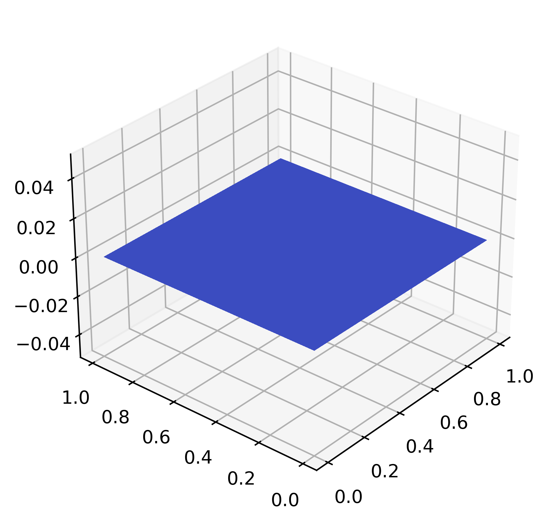
Representative plot at \(t=0\) (left) and \(t=3\), using a 50x50 mesh with Weno5 and RK4 time integration with \(dt = 0.01\), and default values for the physical coefficients: