Governing equations¶

This code simulates the evolution of elastic seismic shear waves in an axisymmetric domain.

Approximating the target body/planet (e.g. Earth) as a sphere, we start from a spherical coordinate system as shown in the figure below:

Continuum Formulation

The axisymmetric approximation implies that fields/quantities are invarint along \(\phi\); therefore, all the derivatives with respect to \(\phi\) can be dropped. The governing equations in the velocity-stress formulation thus reduce to:

\[\large{\rho \frac{\partial v}{\partial t} = \frac{\partial \sigma_{r\phi}}{\partial r} + \frac{\partial \sigma_{\theta\phi}}{r \partial \theta} + \frac{3}{r} \Big(\sigma_{r\phi} + 2 \sigma_{\theta\phi} \cot{\theta} \Big) + f}\]

\[\large{\frac{\partial \sigma_{r\phi}}{\partial t} = G \left( \frac{\partial v}{\partial r} - \frac{1}{r} v \right)}\]

\[\large{\frac{\partial \sigma_{\theta\phi}}{\partial t} = G \left( \frac{1}{r} \frac{\partial v}{\partial \theta} - \frac{\cot{\theta}}{r} v \right)}\]

\(t\) represents time
\(r \in [0, r_{surface}]\) is the radial distance from origin to the surface of the body
\(\theta \in [0, \pi]\) is the polar angle
\(\rho(r, \theta)\) is the density (depends only on the spatial coordinates)
\(v(r, \theta, t)\) is the velocity (for simplicity we drop the subscript, but it is intended to be the \(v_{\phi}\) velocity component)
\(\sigma_{r\phi}(r, \theta, t)\) and \(\sigma_{\theta\phi}(r, \theta, t)\) are the two components of the stress tensor remaining after the axisymmetric approximation
\(f(r, \theta,t)\) is the forcing term
\(G(r, \theta) = v_s^2(r, \theta) \rho(r, \theta)\) is the shear modulus and \(v_s\) being the shear wave velocity (both depend only on the spatial coordinates)

In practice, the axisymmetric approximation means that one solves the above governing equations over a circular sector. Such a formulation is referred to as 2.5-dimensional because it involves a 2-dimensional spatial domain (a circular sector of the Earth) but models point sources with correct 3-dimensional spreading {todo: add citation}.

Semi-discrete System¶

We discretize the 2D spatial domain using a staggered grid, which are typical for seismic modeling and wave problems in general. The figure below shows a sample grid for the Earth (this is just for visualization purposes): the computational domain extends from the surface to the core-mantle boundary, excluding the liquid core.

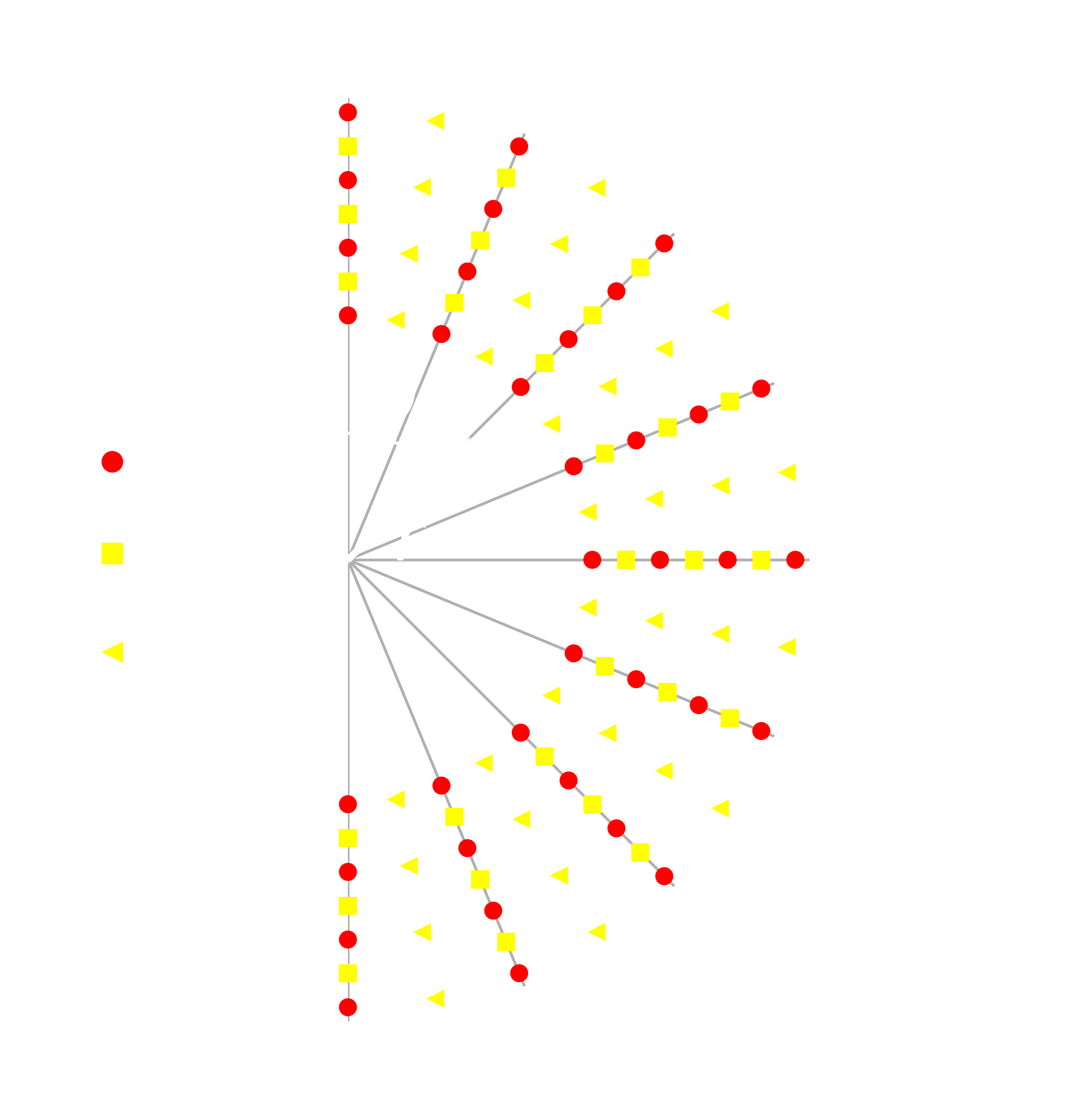
Schematic of the axi-symmetric domain for the Earth and staggered grid used for its discretization. Markers are color-coded to visualize which quantity it represents.¶

In the figure above you notice that the core region is omitted. This is because shear effects are typically negligible in liquids and, therefore, when modeling the Earth, the computational domain is the region bounded between the core-mantle boundary (CMB) located at \(r_{cmb} = 3,480\) km and the Earth surface located at \(r_{earth} = 6,371\) km. When modeling a different body, one needs to use proper domain bounds. Note, however, that the code always assumes the domain NOT to include the singularity at the origin, which yields substantial simplifications.

We use a second-order centered finite-difference method for the spatial operators. This is enough for the purposes of this work. Directly at the symmetry axis, i.e., \(\theta = 0, \pi\), the velocity is set to zero since it undefined here due to the cotangent term in its governing equation. This implies that at the symmetry axis the stress \(\sigma_{r,\phi}\) is also zero. At the core-mantle boundary and earth surface we impose a free surface boundary condition (i.e., waves fully reflect), by setting the zero-stress condition \(\sigma_{r_{cmb},\phi} = \sigma_{r_{earth},\phi} = 0\). Note that this condition on the stress directly defines the velocity at the core-mantle boundary and earth surface and, therefore, no boundary condition on the velocity itself must be set there. Note that we do not rely on ghost points to impose boundary conditions, but account for the boundary conditions directly when assembling the system matrix.

Semi-discrete Rank-1 formulation

\[\large{\frac{d {\boldsymbol x}_{v}}{dt}(t; {\boldsymbol \eta}, {\boldsymbol \mu}) = \mathbf{A}_{v}({\boldsymbol \eta}) {\boldsymbol x}_{\sigma}(t; {\boldsymbol \eta}, {\boldsymbol \mu}) + {\boldsymbol f}_{v}(t; {\boldsymbol \eta}, {\boldsymbol \mu})}\]

\[\large{\frac{d {\boldsymbol x}_{\sigma}}{dt}(t; {\boldsymbol \eta}, {\boldsymbol \mu}) = \mathbf{A}_{\sigma}({\boldsymbol \eta}) {\boldsymbol x}_{v}(t; {\boldsymbol \eta}, {\boldsymbol \mu})}\]

where \({\boldsymbol x}_{v}\) is the state vector for the velocity degrees of freedom, \({\boldsymbol x}_{\sigma}\) is the state vector with the stresses degrees of freedom, \(\mathbf{A}_{v}({\boldsymbol \eta})\) is the discrete system matrix for the velocity, \(\mathbf{A}_{\sigma}({\boldsymbol \eta})\) is the one for the stresses, and \({\boldsymbol f}_{v}(t; {\boldsymbol \eta}, {\boldsymbol \mu})\) is the forcing vector, and \({\boldsymbol \eta}\) are parameters parametrizing the system matrix and \({\boldsymbol \mu}\) are parameters parametrizing the forcing. In this work, the finite difference scheme adopted leads to system matrices \(\mathbf{A}_{v}({\boldsymbol \eta})\) and \(\mathbf{A}_{\sigma}({\boldsymbol \eta})\) with about four and two non-zeros entries per row, respectively.

We refer to this as the rank-1 formulation because the states and forcing are vectors. This solves a single trajectory at a time. One can immediately notice that this formulation is characterized by a standard sparse-matrix vector (spmv) product, which is well-known to be memory bandwidth bound due to its low compute intensity regardless of its sparsity pattern.

Can we develop a more computationally efficient formulation? We can do so as follows: met \({\boldsymbol X}\) represent a set of \(M\) trajectories such that

\[{\boldsymbol X}(t; {\boldsymbol \eta}, \mathcal{M}) \equiv \large[ {\boldsymbol x}_1(t; {\boldsymbol \eta}, {\boldsymbol \mu}_1) \ ... \ {\boldsymbol x}_{M}(t; {\boldsymbol \eta}, {\boldsymbol \mu}_{M}) \large]\]

for a given choice of \({\boldsymbol \eta}\) and where \({\boldsymbol \mu}_1, ..., {\boldsymbol \mu}_{M}\) is the set of parameters defining the \(M\) forcing realizations driving the trajectories of interest. We can then express the dynamics of these \(M\) trajectories as:

Semi-discrete Rank-2 formulation

\[\large{\frac{d {\boldsymbol X}_{v}}{dt}(t; {\boldsymbol \eta}, \mathcal{M}) = \mathbf{A}_{v}({\boldsymbol \eta}) {\boldsymbol X}_{\sigma}(t; {\boldsymbol \eta}, \mathcal{M}) + {\boldsymbol F}_{v}(t; {\boldsymbol \eta}, \mathcal{M})}\]

\[\large{\frac{d {\boldsymbol X}_{\sigma}}{dt}(t; {\boldsymbol \eta}, \mathcal{M}) = \mathbf{A}_{\sigma}({\boldsymbol \eta}) {\boldsymbol X}_{v}(t; {\boldsymbol \eta}, \mathcal{M})}\]

where \({\boldsymbol X}_{v}\) is the rank-2 state tensor for the velocity degrees of freedom, \({\boldsymbol X}_{\sigma}\) is the rank-2 state tensor for the stresses degrees of freedom, \(\mathbf{A}_{v}({\boldsymbol \eta})\) is the discrete system matrix for the velocity, \(\mathbf{A}_{\sigma}({\boldsymbol \eta})\) is the one for the stresses, and \({\boldsymbol F}_{v}(t; {\boldsymbol \eta}, \mathcal{M})\) is the rank-2 forcing tensor. Obviously, the rank-1 formulation can be easily obtained by setting \(M = 1\).

The formulation above has the advantage that it allows us to simulate \(M\) trajectories simultaneously. This now requires a sparse-matrix matrix (spmm) kernel which has a slightly higher higher arithmetic intensity than just spmv, so it has an advantage from a computational standpoint.

Time integration¶

For time integration, we use a leapfrog integrator, where the velocity field is updated first, followed by the stress update. This is a commonly used scheme for classical mechanics because it is time-reversible and symplectic. The initial conditions consist of zero velocity and stresses.