Demo 2

Description:

Simulates the wave dynamic for multiple forcings using the rank-1 formulation and the PREM Earth’s model.

1. Prepare

export SHAWDIR=<fullpath-to-the-source-code-repository>
export EXEDIR=<fullpath-to-where-you-built-the-code-executables>

# create a dir to run the demo
export MYRUNDIR=${HOME}/mySecondDemo
mkdir -p ${MYRUNDIR}

Important

You need to have the code built to proceed, see Building: “expert” mode or Building: step-by-step.

2. Generate the mesh

For this demo, we use a grid of 256 x 1024 velocity points along the radial and polar directions, respectively. To generate the mesh files proceed as follows:

cd ${SHAWDIR}/meshing
python create_single_mesh.py -nr 256 -nth 1024 -working-dir ${MYRUNDIR}

After generating the grid, you should have a ${MYRUNDIR}/mesh256x1024 directory containing:

.
├── [5.9M]  coeff_vp.dat
├── [ 37M]  graph_sp.dat
├── [ 21M]  graph_vp.dat
└── [ 231]  mesh_info.dat

3. Input file

We use the following input file (learn more about input file):

general:
  # meshDir should contain the full path to the mesh directory
  # as generated by the python script `meshing/create_single_mesh.py`
  # but here we use this for simplicity since this input file
  # is used in the doc showing how to run a case
  meshDir: ./mesh256x1024
  dt: 0.25
  finalTime: 2000.0
  checkNumericalDispersion: true
  checkCfl: true

io:
  snapshotMatrix:
    binary: true
    velocity: {freq: 100, fileName: snaps_vp}
    stress:   {freq: 100, fileName: snaps_sp}

  seismogram:
    binary: false
    freq: 4
    receivers: [5,30,55,80,105,130,155,175]

source:
  signal:
    kind: ricker
    depth: [240.,440.,540.,700.]
    period: 65.0
    delay: 180.0

material:
  kind: prem

which we have ready for you to copy as:

cp ${SHAWDIR}/demos/demo2/input.yaml ${MYRUNDIR}

4. Run the simulation

cd ${MYRUNDIR}
ln -s ${EXEDIR}/shawExe .

# if you use OpenMP build, remember to set
# OMP_NUM_THREADS=how-many-you-want-use OMP_PLACES=threads OMP_PROC_BIND=spread
./shawExe input.yaml

You will notice that since we use the rank-1 formulation, the code will solve sequentially all four realizations of the forcing term. To give an idea of runtime, on a MacPro with 2.4 GHz 8-Core Intel Core i9 and 32 GB 2667 MHz DDR4, and using a serial build of the code, each individual realization takes approximately 36 seconds, of which the IO time for data collection is less than 1 second.

5. Simulation data

After running the demo (have some patience because it takes some a couple minutes if you use the serial mode), you should have inside ${MYRUNDIR} the following files:

coords_sp.txt #: coordinates of the velocity grid points
coords_vp.txt #: coordinates of the stresses grid points

seismogram_0  #: seismogram for depth = 240
seismogram_1  #: seismogram for depth = 440
seismogram_2  #: seismogram for depth = 540
seismogram_3  #: seismogram for depth = 700

snaps_vp_0    #: velocity snapshots for depth = 240
snaps_vp_1    #: velocity snapshots for depth = 440
snaps_vp_2    #: velocity snapshots for depth = 540
snaps_vp_3    #: velocity snapshots for depth = 700

snaps_sp_0    #: stresses snapshots for depth = 240
snaps_sp_1    #: stresses snapshots for depth = 440
snaps_sp_2    #: stresses snapshots for depth = 540
snaps_sp_3    #: stresses snapshots for depth = 700

6. Post-process data

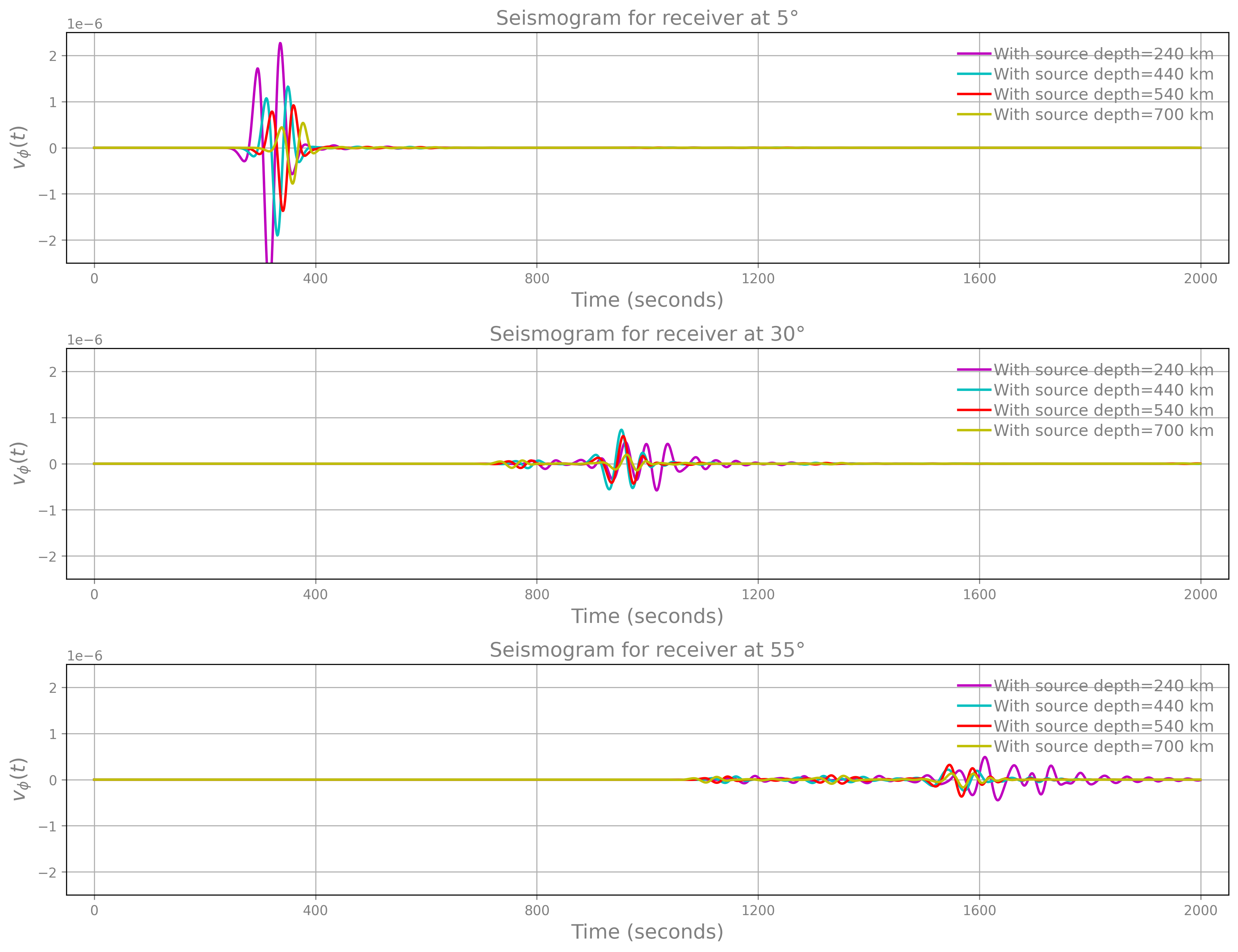
To post-process the data, get the Python scripts created for this demo and visualize the seismogram:

cd ${MYRUNDIR}
cp ${SHAWDIR}/demos/demo2/plotSeismogram.py .
python plotSeismogram.py

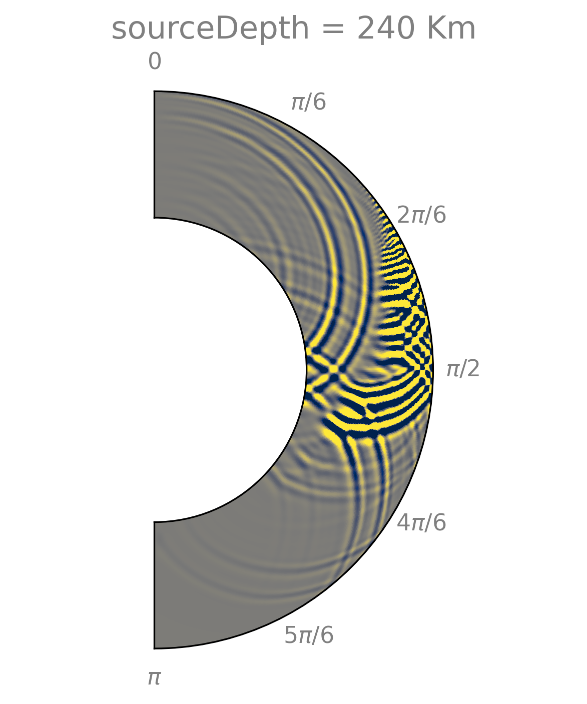
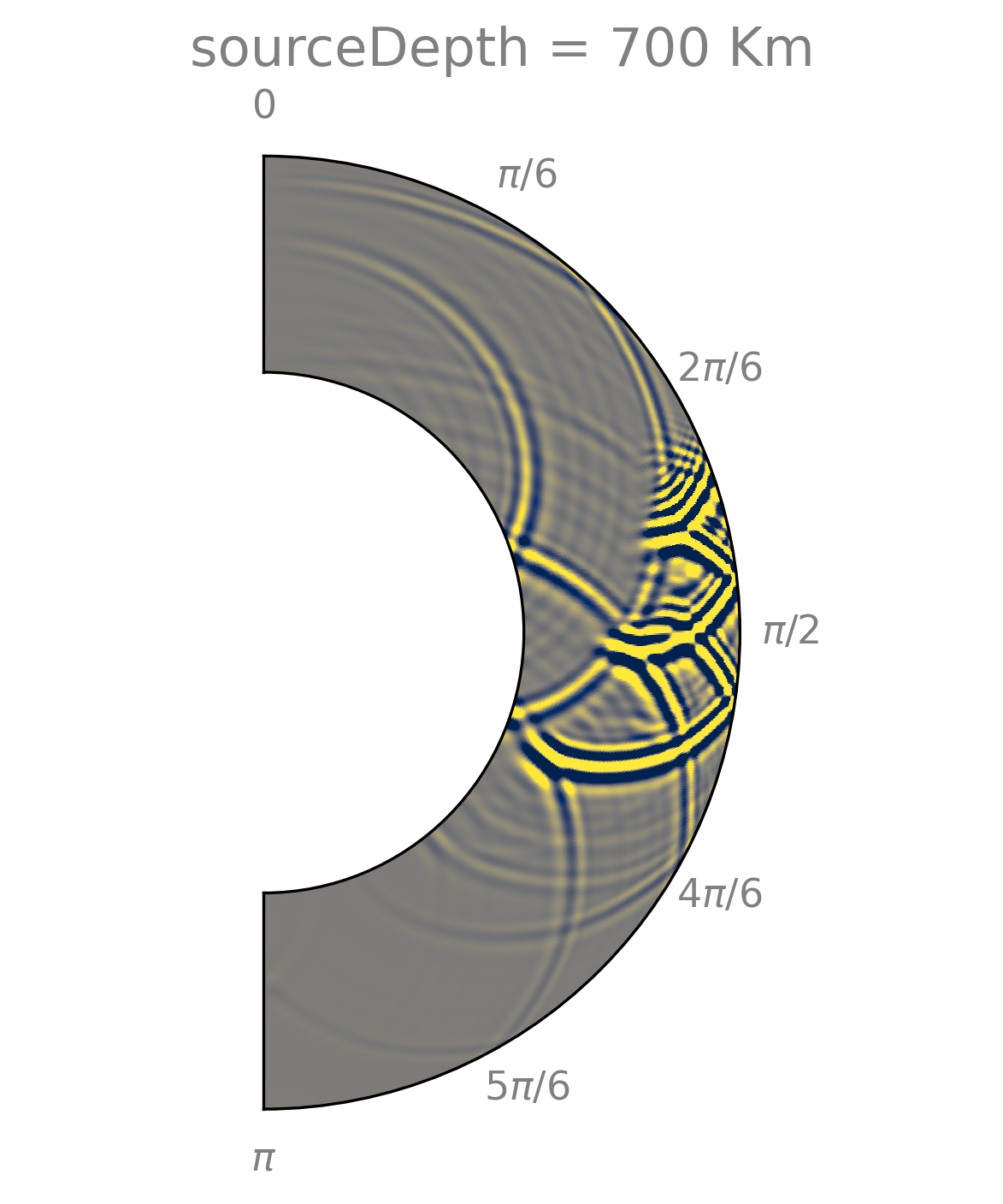
We now extract and compare the velocity wavefield at t=2000 (seconds) for depth=240 and depth=700

cd ${MYRUNDIR}
ln -s ${EXEDIR}/extractStateFromSnaps .

# snaps_vp_0 contains snapshots for depth=240 km
# extract target state and write to file appending vp_d240 to identify the case
./extractStateFromSnaps --snaps=./snaps_vp_0 binary --fsize=1 \
  --outformat=ascii --timesteps=8000  --samplingfreq=100 --outfileappend=vp_d240

# snaps_vp_3 contains snapshots for depth=700 km
# extract target state and write to file appending vp_d700 to identify the case
./extractStateFromSnaps --snaps=./snaps_vp_3 binary --fsize=1 \
  --outformat=ascii --timesteps=8000  --samplingfreq=100 --outfileappend=vp_d700

cp ${SHAWDIR}/demos/demo2/plotWavefield.py .
python plotWavefield.py

And plot them below, showing as expected the largely different pattern and trailing waves due to the complex reflection/refraction effects of the waves propagating through the discontinuous PREM material model.