Demo 3
Description:
Simulates the wave dynamic for multiple forcings using the rank-2 formulation and the PREM Earth’s model. For the sake of demonstration, this demo solves the same problem described in Demo 2, except that here we use the rank-2 formulation, which allows us to simulate several trajectories simultaneously.
1. Prepare
export SHAWDIR=<fullpath-to-the-source-code-repository>
export EXEDIR=<fullpath-to-where-you-built-the-code-executables>

# create a dir to run the demo
export MYRUNDIR=${HOME}/myThirdDemo
mkdir -p ${MYRUNDIR}
Important
You need to have the code built to proceed, see Building: “expert” mode or Building: step-by-step.
2. Generate the mesh
cd ${SHAWDIR}/meshing
python create_single_mesh.py -nr 256 -nth 1024 -working-dir ${MYRUNDIR}
3. Input file
We use the following input file (learn more about input file):
general:
# meshDir should contain the full path to the mesh directory
# as generated by the python script `meshing/create_single_mesh.py`
# but here we use this for simplicity since this input file
# is used in the doc showing how to run a case
meshDir: ./mesh256x1024
dt: 0.25
finalTime: 2000.0
checkNumericalDispersion: true
checkCfl: true
io:
snapshotMatrix:
binary: true
velocity: {freq: 100, fileName: snaps_vp}
stress: {freq: 100, fileName: snaps_sp}
seismogram:
binary: false
freq: 4
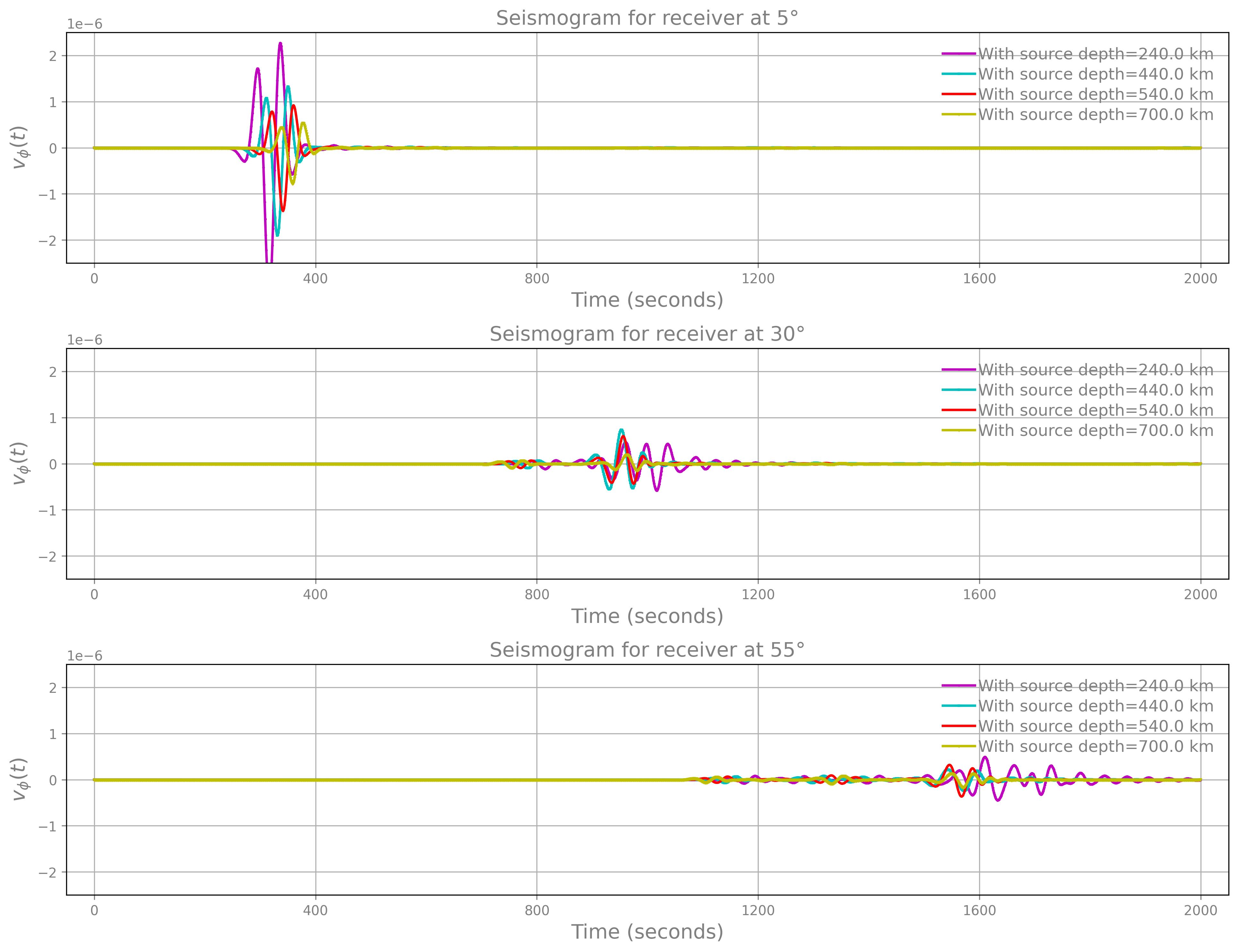
receivers: [5,30,55,80,105,130,155,175]
source:
signal:
kind: ricker
depth: [240.,440.,540.,700.]
period: 65.0
delay: 180.0
forcingSize: 4
material:
kind: prem
which we have ready for you to copy as:
cp ${SHAWDIR}/demos/demo3/input.yaml ${MYRUNDIR}
4. Run the simulation
cd ${MYRUNDIR}
ln -s ${EXEDIR}/shawExe .
./shawExe input.yaml
To give an idea of runtime, on a MacPro with 2.4 GHz 8-Core Intel Core i9 and 32 GB 2667 MHz DDR4, and using a serial build of the code, the run takes approximately 107 seconds, of which the IO time for data collection is less than 1 second. Note that this already gives a hint to the advantages of using the rank-2 formulation. In fact, while here it takes 107 seconds to simulate the four trajectories simultaneously, in rank-1 version of this demo it took about 150 seconds to simulate the same realizations.
5. Simulation data
The demo should generate inside ${MYRUNDIR} the following:
coords_sp.txt #: coordinates of the velocity grid points
coords_vp.txt #: oordinates of the stresses grid points

# seismogram for all forcing realizations at the receiver locations
# the input file set the format to be ascii
# since we have 8 receivers and 4 sample depths, the file generated is as follows:
# rows 1-8  : seismogram for each station when source depth=240 Km
# rows 9-16 : seismogram for each station when source depth=440 Km
# rows 17-24: seismogram for each station when source depth=540 Km
# rows 25-32: seismogram for each station when source depth=700 Km
seismogram_0

snaps_vp_0    #: snapshot matrix for the velocity for all realizations
snaps_sp_0    #: snapshot matrix for the stresses for all realizations
6. Post-process data
To post-process the data, get the Python scripts created for this demo and visualize the seismogram:
cd ${MYRUNDIR}
cp ${SHAWDIR}/demos/demo3/plotSeismogram.py .
python plotSeismogram.py
Which generates a figure identical to the seismogram plot obtained with the rank-1 (as expected) since here we solve the sample problem just in a different, more efficient way.