Demo 1

Description:

Simulates the wave dynamic for a single forcing using the PREM Earth’s model.

1. Prepare

export SHAWDIR=<fullpath-to-the-source-code-repository>
export EXEDIR=<fullpath-to-where-you-built-the-code-executables>

# create a dir to run the demo
export MYRUNDIR=${HOME}/myFirstDemo
mkdir -p ${MYRUNDIR}

Important

You need to have the code built to proceed, see Building: “expert” mode or Building: step-by-step.

2. Generate the mesh

We use a grid of 200 x 1000 velocity points along the radial and polar directions, respectively.

To generate the mesh files proceed as follows:

cd ${SHAWDIR}/meshing
python create_single_mesh.py -nr 200 -nth 1000 -working-dir ${MYRUNDIR}

Note that the grid generator script only needs the velocity points because the stress points are defined automatically based on the staggered scheme.

After generating the grid, you should have a ${MYRUNDIR}/mesh200x1000 directory containing:

.
├── [4.5M]  coeff_vp.dat
├── [ 28M]  graph_sp.dat
├── [ 16M]  graph_vp.dat
└── [ 231]  mesh_info.dat

3. Input file

We use the following input file (learn more about input file):

general:
  meshDir: ./mesh200x1000
  dt: 0.25
  finalTime: 2000.0
  checkNumericalDispersion: true
  checkCfl: true

io:
  snapshotMatrix:
    binary: true
    velocity:
      freq: 100
      fileName: snaps_vp
    stress:
      freq: 100
      fileName: snaps_sp

  seismogram:
    binary: false
    freq: 4
    receivers:
    - 5
    - 30
    - 80

source:
  signal:
    kind: ricker
    depth: 640.0
    period: 65.0
    delay: 180.0

material:
  kind: prem

which we have ready for you to copy as:

cp ${SHAWDIR}/demos/demo1/input.yaml ${MYRUNDIR}

4. Run the simulation

cd ${MYRUNDIR}

# soft link the executable
ln -s ${EXEDIR}/shawExe .

# if you use OpenMP build, remember to set
# OMP_NUM_THREADS=how-many-you-want-use OMP_PLACES=threads OMP_PROC_BIND=spread
./shawExe input.yaml

5. Post-process data

The demo should generate inside ${MYRUNDIR} the following:

coords_sp.txt #: coordinates of the velocity grid points
coords_vp.txt #: coordinates of the stresses grid points
seismogram_0  #: seismogram at the receiver locations set in input.yaml
snaps_vp_0    #: snapshot matrix for the velocity
snaps_sp_0    #: snapshot matrix for the stresses

We created Python scripts for this:

cp ${SHAWDIR}/demos/demo1/*.py ${MYRUNDIR}

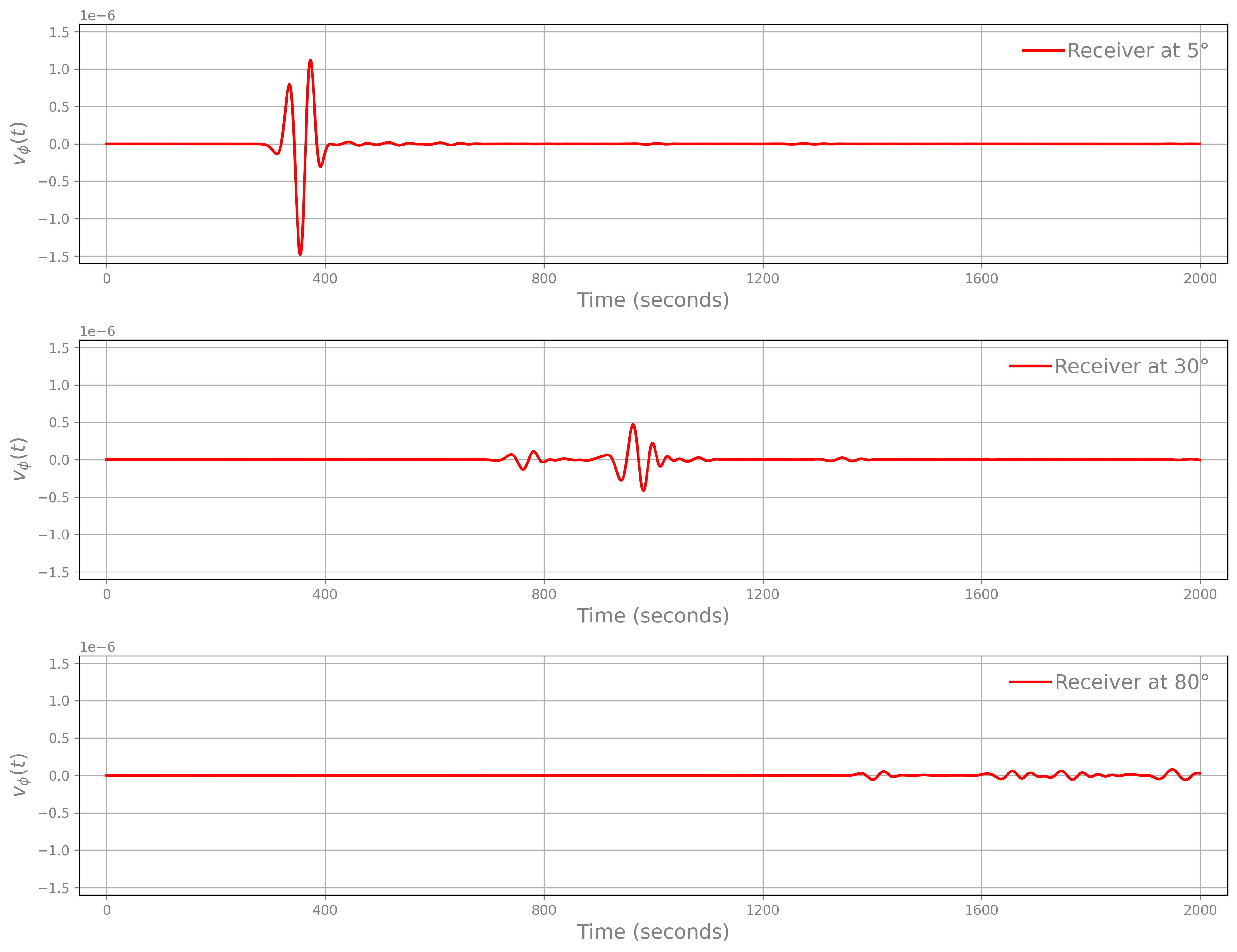
First, the seismogram data:

cd ${MYRUNDIR}
python plotSeismogram.py

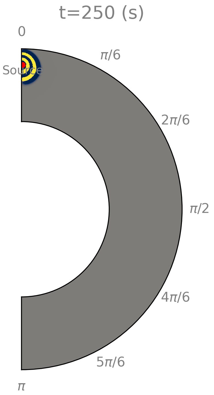
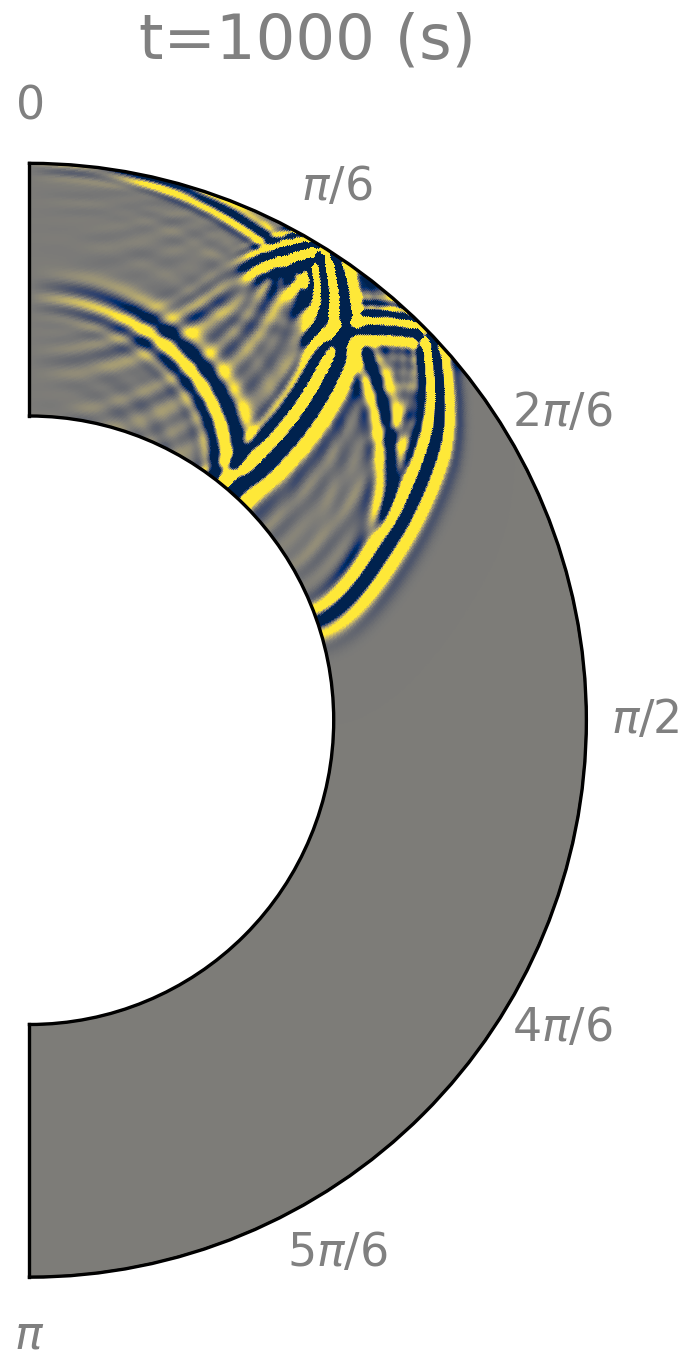
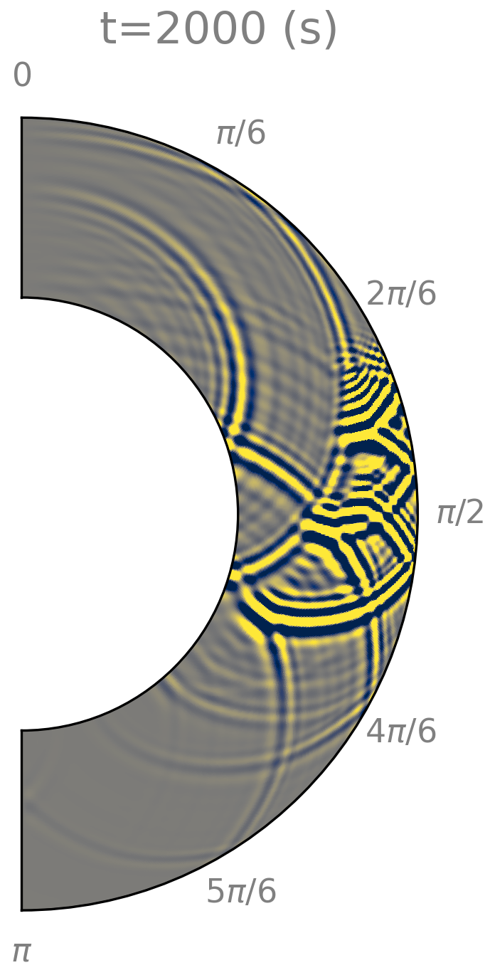
Then, contour plots of the velocity field at t=250, 1000, 2000 (seconds):

cd ${MYRUNDIR}
ln -s ${EXEDIR}/extractStateFromSnaps .

# extract from the velocity snapshots the velocity field at specific timesteps:
# since we use ``dt = 0.25`` seconds, our tartgets ``t=250, 1000, 2000``,
# correspond to *time steps* 1000, 4000, 8000
./extractStateFromSnaps --snaps=./snaps_vp_0 binary --fsize=1 \
  --outformat=ascii --timesteps=1000 4000 8000 \
  --samplingfreq=100 --outfileappend=vp

python plotWavefield.py