Solid dynamics example gallery

The figures on this page are generated from the example implementations during the documentation build. The setup schematics are drawn programmatically and the response figures and animation use trajectories produced by the actual solid-dynamics solver.

Cantilever beam

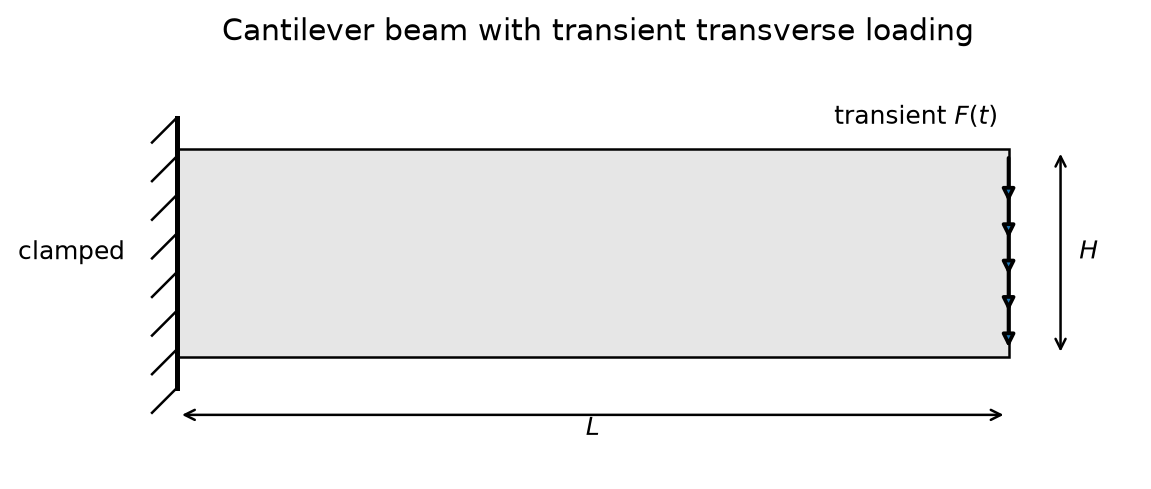
The cantilever example clamps the left boundary and applies a smooth transient transverse resultant on the right boundary.

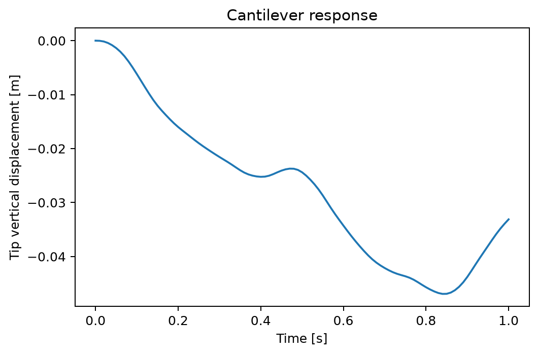
The vertical displacement history at the midpoint of the free end is computed with the default Neo-Hookean model and velocity-primary implicit Newmark solver. No artificial damping is enabled in the default example.

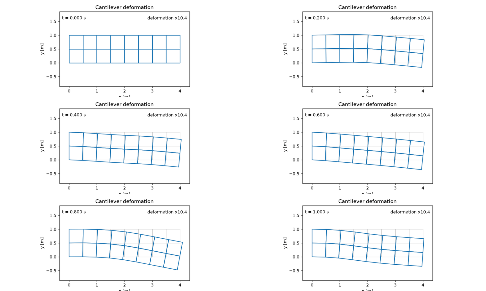
The full displacement snapshots can also be viewed as a deformed-mesh animation. The displayed deformation is magnified when needed for visibility; the magnification factor is shown in the animation.

Doubly clamped Gaussian perturbation

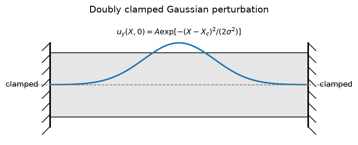
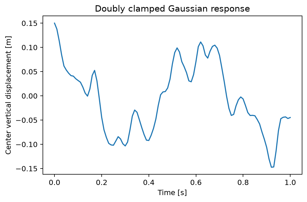
The second example fixes both ends and initializes a centered transverse Gaussian displacement. It is unforced after release.

The following curve is the center-point vertical displacement produced by the Neo-Hookean solver. Because the example has no Rayleigh damping, changes in the center-point amplitude reflect nonlinear and multimode dynamics rather than an imposed damping model.

Longitudinal two-way wave

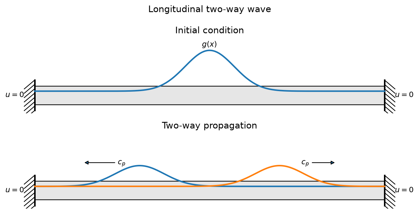
For the linear-wave verification problem, all transverse degrees of freedom are constrained and an axial Gaussian displacement is released from rest. Before boundary reflections, the solution reduces to the scalar two-way wave equation.

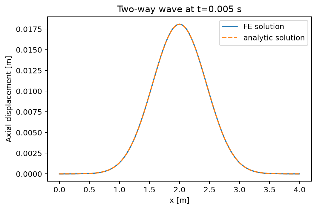
The finite-element solution is compared directly with the analytic D’Alembert solution at the same time.

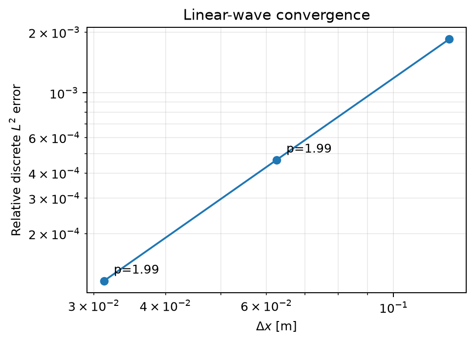
A coupled spatial/temporal refinement study with \(\Delta t\propto\Delta x\) shows the expected near-second-order convergence.

Generation

All media on this page are regenerated by examples/nonlinear_solid_dynamics/generate_docs_media.py during the Sphinx build. This keeps the visualizations tied to the current solver rather than maintaining hand-generated result images.