HIFiRE-1#
One of our driving use cases for Pressio is for simulations of hypersonic aerodynamics. Model reduction is necessary because computational models are widely used in the hypersonic flight regime due to the expense and difficulty of flight tests and experiments. The reliance on computational models as well as the risk tolerances in hypersonic applications requires a greater emphasis on trustworthiness of these models. Unfortunately, crucial tasks including parameter calibration, uncertainty/error propogation, and (robust) design optimization require many model evalutations.
Model reduction with Pressio enables these many query analysis for higher fidelity aerodynamic simulations such as finite volume models of the Navier-Stokes and Reynolds-Averaged Navier–Stokes (RANS) equations. The following section contains results obtained using Pressio and the Sandia Aerodynamics and Reentry Code (SPARC) [Howard et al. 2017][1]. The results shown below are presented in greater detail in [Blonigan et al. 2021][2].
Description#
The HiFIRE-1 (Hypersonic International Flight Research Experimentation) vehicle was an instrumented sounding rocket flown to collect data on hypersonic boundary layer transition [Kimmeland and Adamczak, 2012][3]. We consider a high-fidelity RANS simulation of the payload shown below in the 3D rendering:
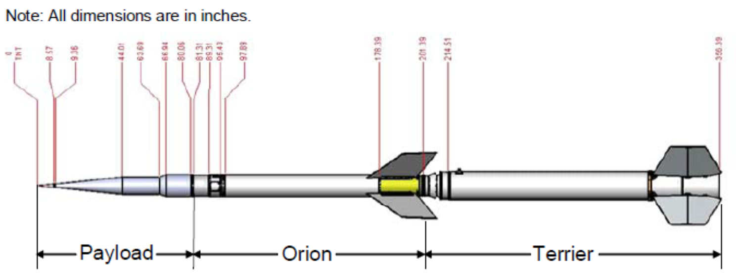
HIFiRE-1 booster stack [Kimmeland and Adamczak, 2012][3]#
The range of flight conditions used in our simulations are chosen to be similar to the flow conditions of a wind tunnel test of HiFIRE-1, specfically run 34 of the experimental campaign undertaken at the CALSPAN University of Buffalo Research Center (CUBRC) [Wadhams et al., 2008][4]. A table with wind tunnel conditions corresponding to run 34 is included below:
Density |
\(0.070215 kg/m^3\) |
Velocity |
\(2168.7 m/s\) |
Mach Number |
\(7.1\) |
Angle of attack |
\(2.0^{\circ}\) |
Temperature |
\(231.91 K\) |
Reynolds Number |
\(1e7 1/m\) |
For this case, turbulent transition is modeled by tripping the boundary layer 0.35 m downstream from the leading edge of the vehicle.
Full order model (FOM)#
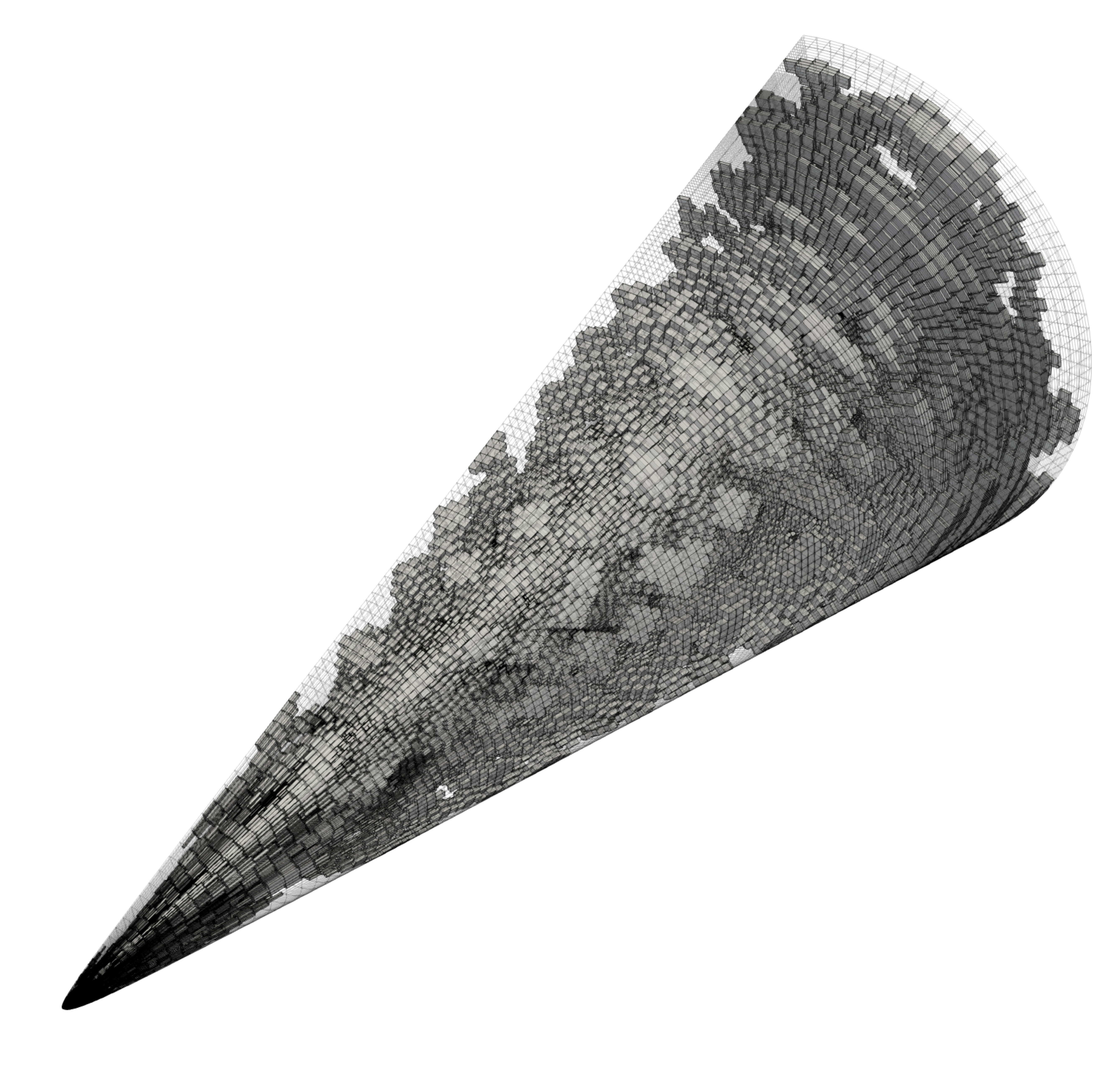
Since the HIFiRE-1 payload geometry is axisymmetric, but the angle of attack is non-zero, we assume symmetry about the centerline anduse the half mesh shown below
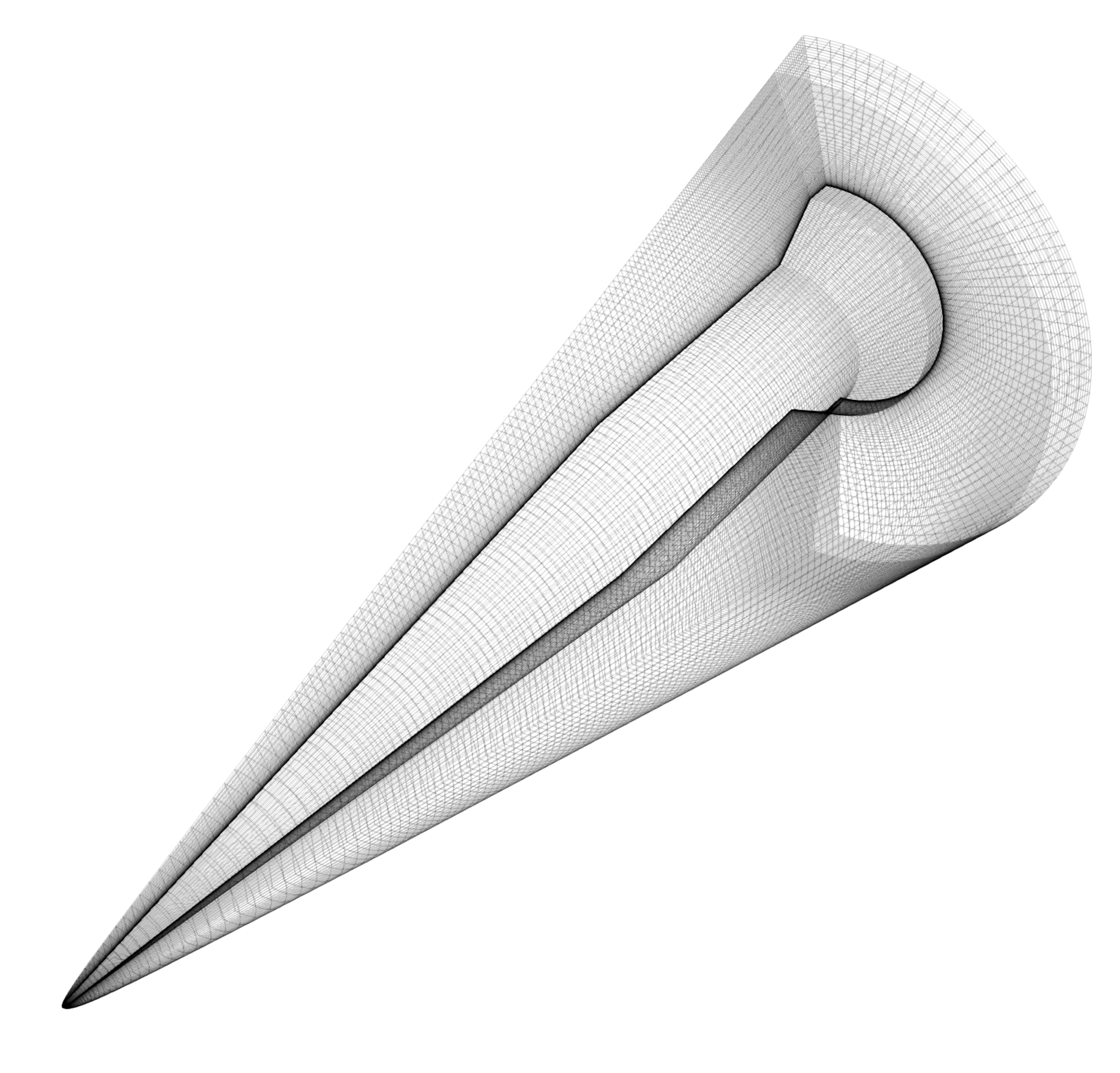
HIFiRE-1 mesh [Blonigan et al., 2021][2]#
The mesh has 2,031,616 cells, corresponding to a state-space size of 12,189,696 since we are using the one-equation Spalart-Allmaras turbulence model. The FOMs were solved to a steady state using pseudo time stepping with a backward Euler integration scheme. The stopping criteria were a 5 order of magnitude.
A total of 36 FOMs are run at the sample points shown below
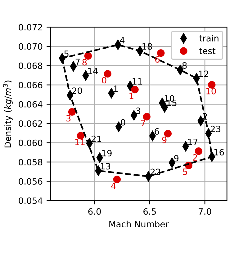
FOM samples [Blonigan et al., 2021][2]#
The 24 FOMs labeled “train” are used to construct a POD basis for the ROM; the FOMs labeled “test” are used to compare the ROM against. The plots below show several flow solutions.
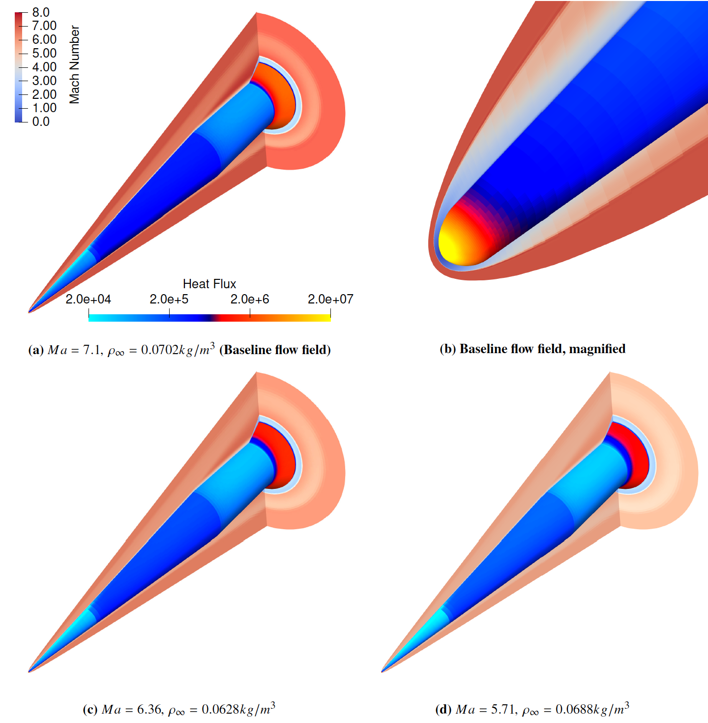
FOM solutions colored by Mach number and wall heat flux [Blonigan et al., 2021][2]#
The main feature of the flow field include a bow shock near the nose, an expansion wave just aft of the cone and an oblique shock upstream of the flange. Boundary layer transition is visible in the sudden jump in heat flux.
LSPG ROM#
Method#
We use a Least-Squares Petrov–Galerkin (LSPG) ROM with a conservation constraint at the 12 test conditions shown previously. The conservation constraint is applied to the entire volume, as discussed in section III.B of [Blonigan et al. 2021][2]. The constrained LSPG solver is implemented using a customized nonlinear solver in Pressio. The solver is run until the relative residual of the normal equations is reduced by 5 orders of magnitude. The initial guess for the ROM generalized coordinates were computed with inverse distance interpolation as suggested by Washabaugh (Algorithm 23) [Washabaugh 2016][5]. The basis is constructed from the leading 4 POD modes computed from all 24 training snapshots. The POD modes are scaled to account for the different magnitudes of each conserved quantity; see section IV.C of [Blonigan et al. 2021][2] for more details of the ROM method.
TODO more details on what features of Pressio are used?
Hyper-reduction is achieved using a sample mesh composed of 16,253 randomly selected cells in which the residual is sampled, along with neighboring cells and neighbors of neighbors, yielding 364,468 cells in total, equivalent to roughly 17.9% of the full mesh. It is shown below:
Sample mesh used for the ROM.#
Results#
Using this sample mesh resulted in a ROM with a speed-up of 300-1,000; that is, around 300-1,000 ROMs could be run with the computational resources required for a single FOM. This substantial cost reduction comes with almost no loss in accuracy: a maximum state error of around than 0.3% across all 12 test cases, as well as errors of no more than 3% in integrated wall heat flux.
TODO ROM vs. FOM flow visualization(s)
The following figure shows the error of the wall pressure and heat flux computed by the ROM for test case 10.
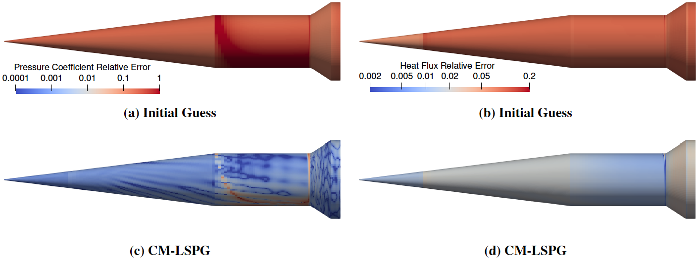
The ROM computes the surface quantities with errors of 1-3% or less over most of the vehicle surface. This is substantially more accurate surface quantities than the interpolation used for the initial guess shown on top.
Additional results can be found in [Rizzi et al. 2020][3].
Tip
ROMs are low cost and accurate
A hyper-reduced ROM produces results within 1% of the full model results, but only requires around 1% of the computational resources needed for the full model.
References#
[1]: Micah Howard, Andrew Bradley, Steven W. Bova, James Overfelt, Ross Wagnild, Derek Dinzl, Mark Hoemmen and Alicia Klinvex. “Towards Performance Portability in a Compressible CFD Code,” AIAA 2017-4407. 23rd AIAA Computational Fluid Dynamics Conference. June 2017.
[2]: Patrick J. Blonigan, Francesco Rizzi, Micah Howard, Jeffrey A. Fike, and Kevin T. Carlberg, Model Reduction for Steady Hypersonic Aerodynamics via Conservative Manifold Least-Squares Petrov–Galerkin Projection, AIAA Journal 2021 59:4, 1296-1312
[3]: Roger Kimmel and David Adamczak. “HIFiRE-1 Background and Lessons Learned,” AIAA 2012-1088. 50th AIAA Aerospace Sciences Meeting including the New Horizons Forum and Aerospace Exposition. January 2012.
[4]: Wadhams, T. P., Mundy, E., MacLean, M. G., and Holden, M. S., “Ground Test Studies of the HIFiRE-1 Transition Experiment Part 1: Experimental Results,” Journal of Spacecraft and Rockets, Vol. 45, No. 6, 2008, pp. 1134–1148.
[5]: K. M. Washabaugh, “Fast Fidelity for Better Design: A Scalable Model Order Reduction Framework for Steady Aerodynamic Design Applications”, PhD Thesis, Department of Aeronautics and Astronautics, Stanford University, August 2016.