Analytic sine VI and MF-VI examples#
These examples use the analytically tractable sine-series inverse problem from the VI/MF-VI benchmark. The forward model is
with
so the exact solution is
The prior is
with synthetic truth
and observation-noise standard deviation \(\sigma_\eta=5\times10^{-3}\). Because the forward map is linear and the prior and likelihood are Gaussian, the exact posterior is available in closed form,
This lets both examples measure convergence directly against the exact posterior.
VI-paper benchmark configuration#
The diagonal example uses the Newton and multifidelity settings from the VI-paper analytic-sine benchmark. The production run uses a full Hessian, lagged stochastic curvature with averaging factor \(\beta=0.25\), natural coordinates, and the paper line-search scales:
optimizer = VINewtonOptimizerConfig(
    newton_metric="natural",
    newton_hessian_type="full",
    newton_curvature_strategy="lagged",
    newton_hessian_averaging_factor=0.25,
    newton_regularization=5e-4,
    gradient_norm_tolerance=0.0,
    max_iterations=1000,
)

line_search = VIStochasticNonmonotoneLineSearchConfig(
    initial_step_size=0.25,
    max_step_size=1.0,
)
The shared VI/MF-VI arguments use the joint entropy estimator, a leave-one-out baseline, zero observation-covariance regularization, and inference seed 7. MF-VI uses a scalar multifidelity control-variate coefficient in both examples:
common_arguments = dict(
    ...,
    optimizer_method="newton",
    optimizer_config=optimizer,
    line_search_method="stochastic_nonmonotone",
    line_search_config=line_search,
    baseline_method="loo",
    score_function_entropy_strategy="joint",
    covariance_regularization=0.0,
    random_seed=7,
)
The full diagonal run uses 16 FOM samples per iteration. MF-VI uses 64 additional ROM samples, the automatic GP ROM, and four iterations of ROM training history:
workflows.mf_vi_with_auto_rom(
    ...,
    fom_sample_size=16,
    rom_extra_sample_size=64,
    max_rom_training_history=4,
    mfmc_control_variate_mode="scalar",
    rom_type="gp",
    rom_args={
        "normalize_parameters": True,
        "normalize_targets": True,
    },
)
prior_parameter_space defines the Bayesian prior, while the required
initial_variational_parameter_space independently selects the variational
family and supplies its initial moments.
Example 1: equispaced observations and a diagonal posterior#
The first example uses \(N=31\) equispaced interior observations,
For these points the discrete sine basis is orthogonal, so \(G^T\Gamma_{\rm obs}^{-1}G\) is diagonal. Since the prior covariance is also diagonal, the exact posterior covariance is diagonal to numerical precision.
The variational initializer is a GaussianParameterSpace. This selects the
diagonal/mean-field VI implementation. This is the case that corresponds
directly to the VI-paper analytic-sine benchmark and therefore uses the exact
configuration listed above.
Run the example with
python examples/vi_mf_vi_demo/diagonal_example.py
Convergence#
The convergence plot reports the exact Gaussian \(D_{\rm KL}(q\|p_{\rm post})\) for the accepted VI and MF-VI states.
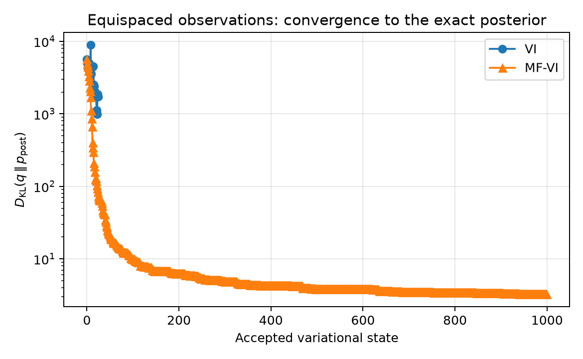
VI and MF-VI convergence to the exact diagonal posterior.#
Posterior mean#
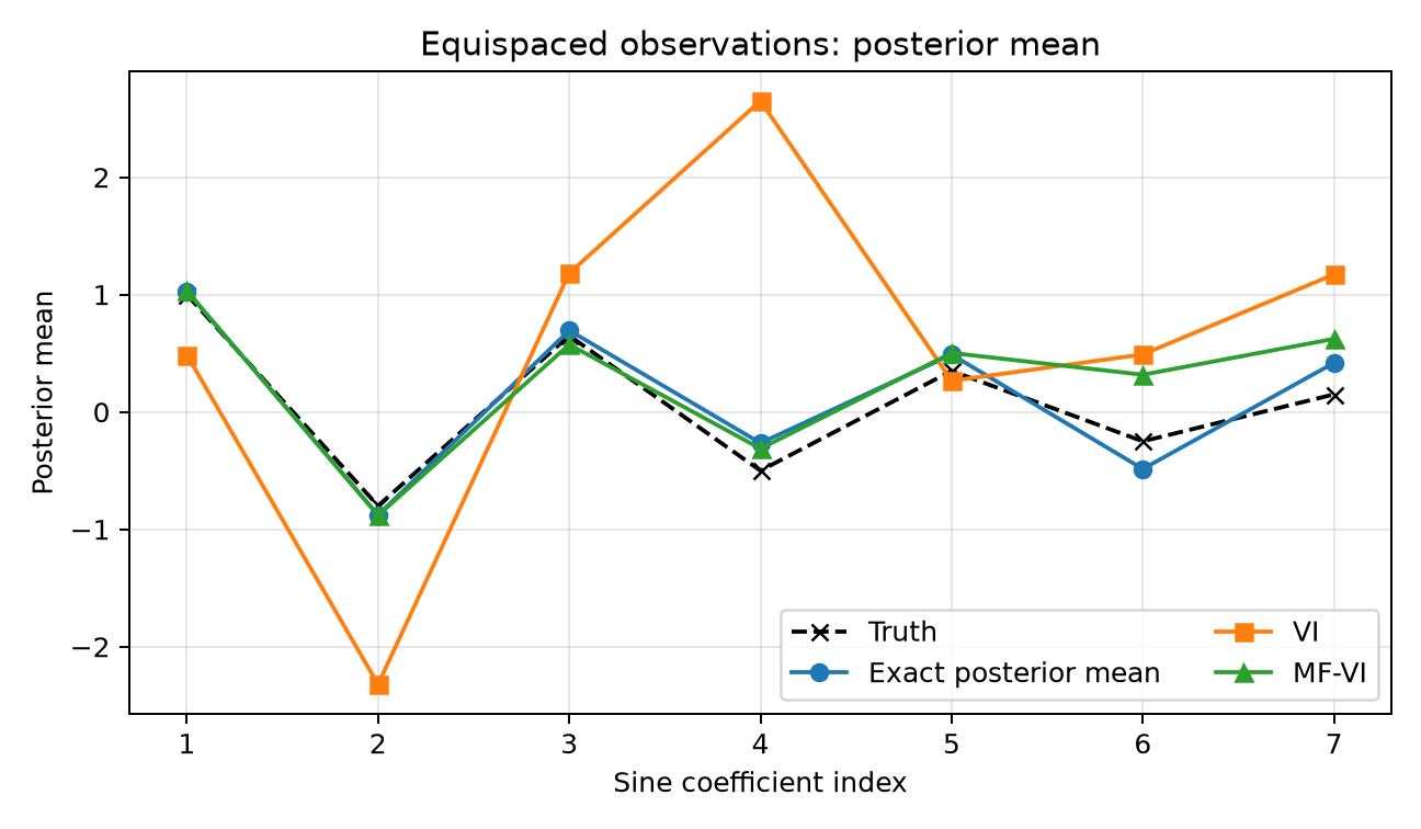
Final VI and MF-VI posterior means compared with the exact posterior mean and the synthetic truth.#
Posterior#
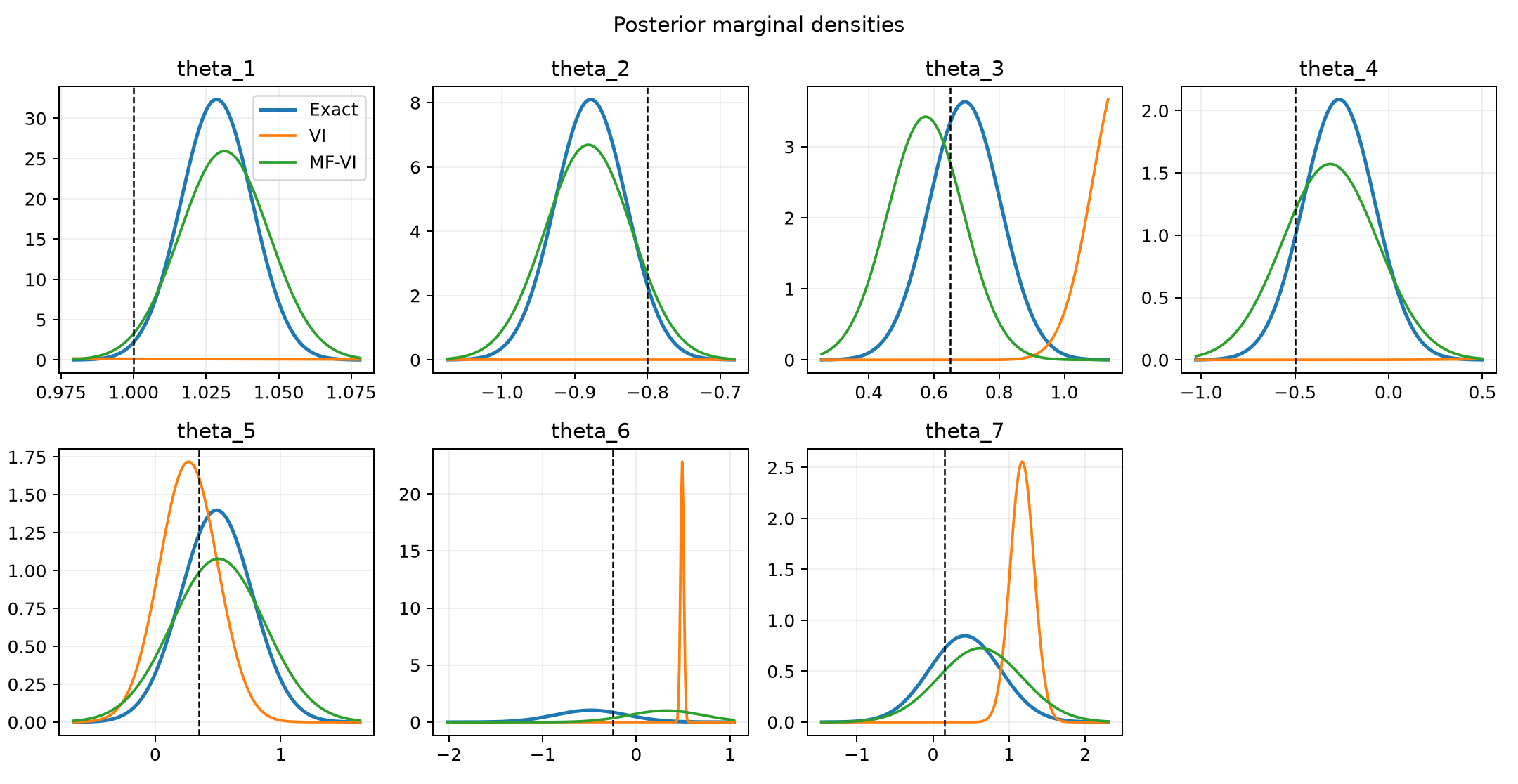
Exact, VI, and MF-VI marginal posterior densities for the seven sine coefficients. The vertical dashed line in each panel is the synthetic truth.#
Implementation#
  1"""VI versus MF-VI for the diagonal analytic sine posterior."""
  2
  3from __future__ import annotations
  4
  5import argparse
  6from pathlib import Path
  7import shutil
  8import sys
  9from typing import Optional
 10
 11import numpy as np
 12
 13
 14REPOSITORY_ROOT = Path(__file__).resolve().parents[2]
 15if str(REPOSITORY_ROOT) not in sys.path:
 16    sys.path.insert(0, str(REPOSITORY_ROOT))
 17
 18import romtools.workflows as workflows
 19from romtools.workflows.inverse.vi_optimization_methods import (
 20    VINewtonOptimizerConfig,
 21    VIStochasticNonmonotoneLineSearchConfig,
 22)
 23from romtools.workflows.parameter_spaces import GaussianParameterSpace, MonteCarloSampler
 24
 25from examples.vi_mf_vi_demo.analytic_sine_support import (
 26    AnalyticSineQoiModel,
 27    PRIOR_STD,
 28    build_problem,
 29    collect_history,
 30    write_convergence_plot,
 31    write_diagonal_posterior_plot,
 32    write_mean_plot,
 33)
 34
 35
 36def main(
 37    smoke: bool = False,
 38    work_dir: Optional[str] = None,
 39    output_dir: Optional[str] = None,
 40) -> None:
 41    """Run the equispaced-observation diagonal-posterior example."""
 42    problem = build_problem(equispaced=True)
 43    model = AnalyticSineQoiModel(problem)
 44
 45    sample_size = 8 if smoke else 16
 46    rom_extra_sample_size = 8 if smoke else 64
 47    max_iterations = 2 if smoke else 1000
 48
 49    prior = GaussianParameterSpace(
 50        parameter_names=list(problem.parameter_names),
 51        means=problem.prior_mean,
 52        stds=np.full(problem.prior_mean.size, PRIOR_STD),
 53        sampler=MonteCarloSampler,
 54    )
 55    initial_variational_parameter_space = GaussianParameterSpace(
 56        parameter_names=list(problem.parameter_names),
 57        means=problem.prior_mean,
 58        stds=np.full(problem.prior_mean.size, PRIOR_STD),
 59        sampler=MonteCarloSampler,
 60    )
 61    optimizer = VINewtonOptimizerConfig(
 62        newton_metric="natural",
 63        newton_hessian_type="full",
 64        newton_curvature_strategy="lagged",
 65        newton_hessian_averaging_factor=0.25,
 66        newton_regularization=5e-4,
 67        gradient_norm_tolerance=0.0,
 68        max_iterations=max_iterations,
 69    )
 70    line_search = VIStochasticNonmonotoneLineSearchConfig(
 71        initial_step_size=0.25,
 72        max_step_size=1.0,
 73    )
 74
 75    root = (
 76        Path(work_dir).resolve()
 77        if work_dir
 78        else Path(__file__).parent / "diagonal_work"
 79    )
 80    shutil.rmtree(root, ignore_errors=True)
 81    vi_dir = root / "vi"
 82    mf_vi_dir = root / "mf_vi"
 83
 84    common_arguments = dict(
 85        model=model,
 86        prior_parameter_space=prior,
 87        initial_variational_parameter_space=initial_variational_parameter_space,
 88        observations=problem.observations,
 89        observations_covariance=problem.observation_covariance,
 90        optimizer_method="newton",
 91        optimizer_config=optimizer,
 92        line_search_method="stochastic_nonmonotone",
 93        line_search_config=line_search,
 94        baseline_method="loo",
 95        score_function_entropy_strategy="joint",
 96        bounded_parameter_handling="clip",
 97        covariance_regularization=0.0,
 98        random_seed=7,
 99        restart_files_to_keep=max_iterations + 1,
100    )
101
102    workflows.run_vi(
103        **common_arguments,
104        absolute_work_dir=str(vi_dir),
105        sample_size=sample_size,
106        evaluation_concurrency=1,
107    )
108    workflows.mf_vi_with_auto_rom(
109        **common_arguments,
110        absolute_work_dir=str(mf_vi_dir),
111        fom_sample_size=sample_size,
112        rom_extra_sample_size=rom_extra_sample_size,
113        fom_evaluation_concurrency=1,
114        rom_evaluation_concurrency=1,
115        max_rom_training_history=4,
116        mfmc_control_variate_mode="scalar",
117        rom_type="gp",
118        rom_args={
119            "normalize_parameters": True,
120            "normalize_targets": True,
121        },
122    )
123
124    vi_history = collect_history(vi_dir, problem)
125    mf_history = collect_history(mf_vi_dir, problem)
126    output = (
127        Path(output_dir).resolve()
128        if output_dir
129        else Path(__file__).parent
130    )
131    write_convergence_plot(
132        output / "analytic_sine_diagonal_convergence.png",
133        vi_history,
134        mf_history,
135        "Equispaced observations: convergence to the exact posterior",
136    )
137    write_mean_plot(
138        output / "analytic_sine_diagonal_mean.png",
139        problem,
140        vi_history,
141        mf_history,
142        "Equispaced observations: posterior mean",
143    )
144    write_diagonal_posterior_plot(
145        output / "analytic_sine_diagonal_posterior.png",
146        problem,
147        vi_history,
148        mf_history,
149    )
150
151
152def _parse_args():
153    parser = argparse.ArgumentParser(description=__doc__)
154    parser.add_argument("--smoke", action="store_true")
155    parser.add_argument("--work-dir")
156    parser.add_argument("--output-dir")
157    return parser.parse_args()
158
159
160if __name__ == "__main__":
161    arguments = _parse_args()
162    main(
163        smoke=arguments.smoke,
164        work_dir=arguments.work_dir,
165        output_dir=arguments.output_dir,
166    )
Example 2: non-equispaced observations and a correlated posterior#
The second example keeps the same model, prior, truth, noise level, and number of observations, but changes only the observation locations. Starting from
the locations are warped according to
This breaks discrete sine orthogonality. The exact posterior therefore has nonzero cross-covariances (the largest absolute posterior correlation is about 0.30 for this setup).
The prior remains the same diagonal GaussianParameterSpace. The primary
full-covariance runs use a MultivariateGaussianParameterSpace initialized
with the same diagonal prior covariance. Its type selects true
full-covariance VI, allowing off-diagonal covariance entries to develop during
optimization. The same correlated target is also solved with a
GaussianParameterSpace variational initializer for both VI and MF-VI. Those
additional mean-field runs deliberately prohibit cross-covariances and expose
the approximation error caused by the restricted variational family.
All four runs retain the same natural Newton metric, full Hessian, lagged curvature with \(\beta=0.25\), line-search scales, random seed, and sample allocation: 16 FOM samples per iteration and 64 additional ROM samples for MF-VI. MF-VI uses the same GP configuration, four iterations of ROM training history, and scalar multifidelity control variate for both variational families. The production optimization budget is 80 iterations. Regular VI uses Newton regularization \(5\times10^{-4}\), while MF-VI uses \(1\times10^{-4}\).
For the full-covariance family, Newton curvature is formed in \((\mu,\operatorname{svec}(\Sigma))\) coordinates and locally whitened with the exact Gaussian Fisher metric before the regularized Newton solve. The covariance update is then applied with the SPD-preserving exponential retraction described in Full-covariance variational inference.
Run the example with
python examples/vi_mf_vi_demo/full_covariance_example.py
Convergence#
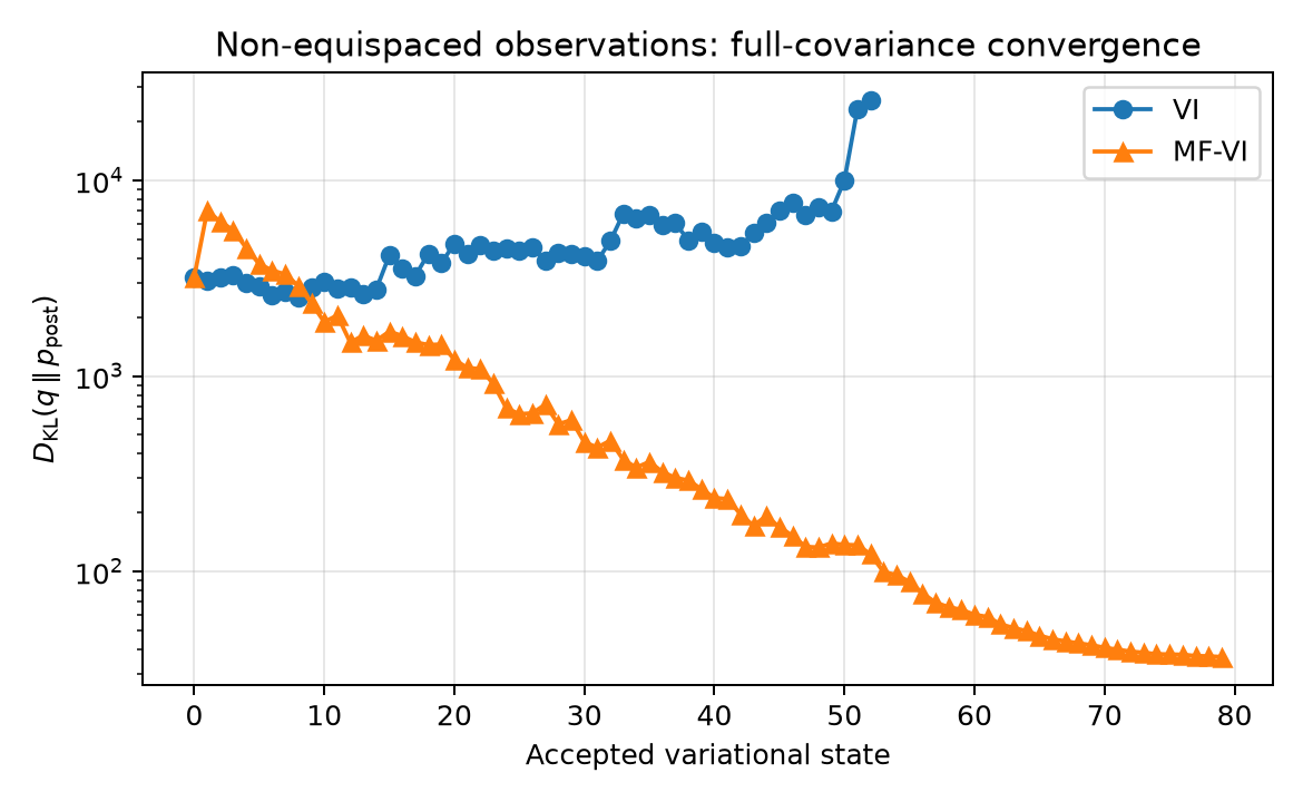
Exact Gaussian KL convergence for full-covariance VI and MF-VI.#
Posterior mean#
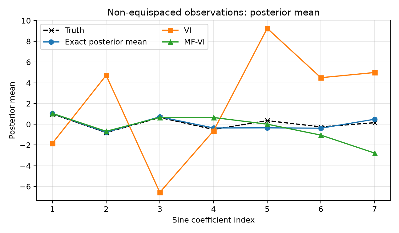
Final full-covariance VI and MF-VI posterior means compared with the exact posterior mean and truth.#
Posterior#
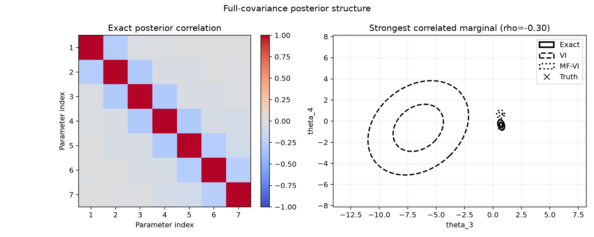
The exact posterior correlation matrix and the strongest correlated two-dimensional marginal. The ellipse panel compares one- and two-standard-deviation contours from the exact posterior, full-covariance VI, and full-covariance MF-VI.#
Variational-family error#
Because the target is Gaussian, the best possible reverse-KL mean-field approximation is known analytically. If \(P_{\rm post}=C_{\rm post}^{-1}\), the optimum over diagonal Gaussian covariances has
Its nonzero \(D_{\rm KL}(q\|p_{\rm post})\) therefore provides an exact variational-family error floor. The next plot overlays the full-covariance and mean-field VI/MF-VI histories and marks this floor. A mean-field method that converges to the horizontal line has exhausted its optimization error; the remaining KL discrepancy is caused by the diagonal covariance restriction.
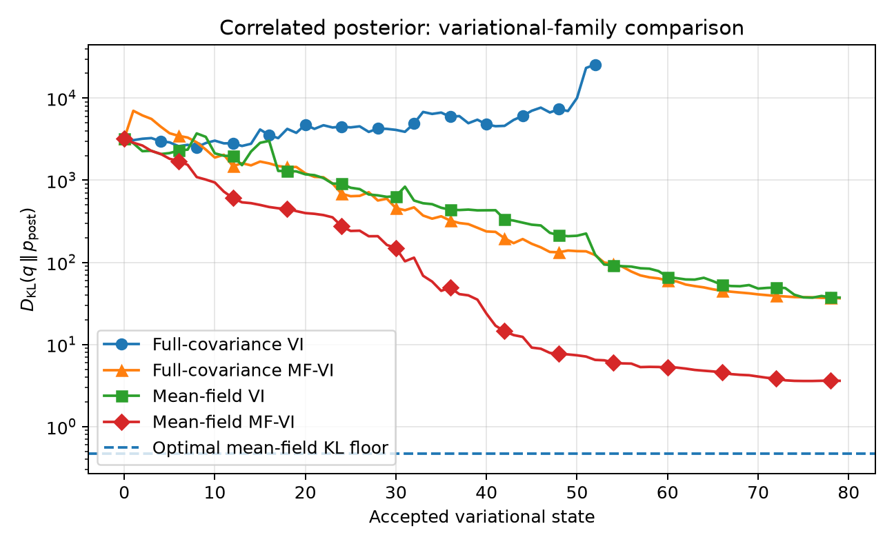
Full-covariance and mean-field VI/MF-VI convergence on the same correlated target. The dashed horizontal reference is the exact optimal mean-field KL floor.#
The covariance restriction is also visible directly in posterior correlation. The exact target and full-covariance approximations can represent the induced cross-correlations, whereas the optimal mean-field approximation and both mean-field numerical runs are diagonal by construction.
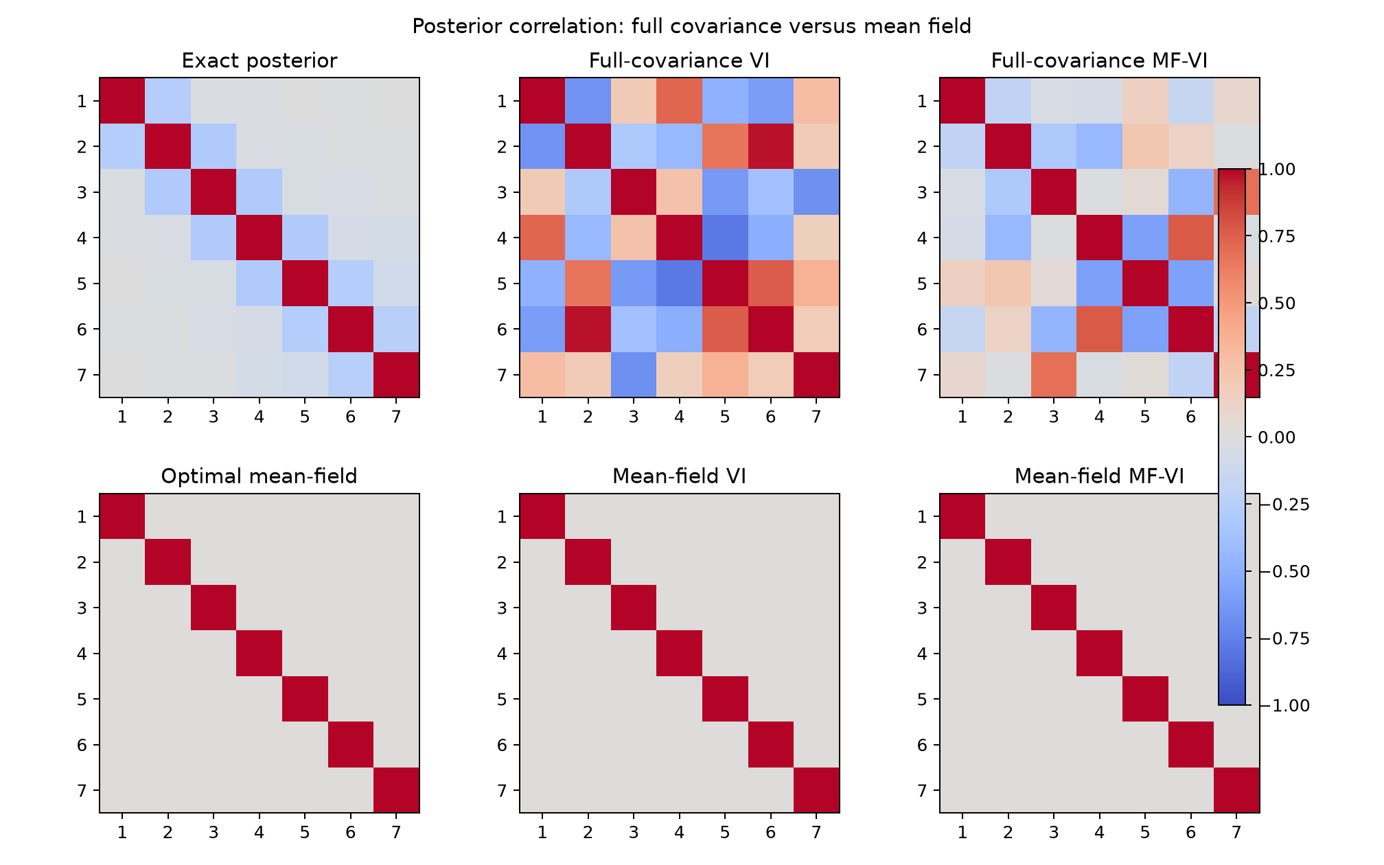
Posterior correlation matrices for the exact target, full-covariance VI and MF-VI, the analytic optimal mean-field approximation, and mean-field VI and MF-VI.#
Implementation#
  1"""Full- and mean-field VI/MF-VI for non-equispaced sine observations."""
  2
  3from __future__ import annotations
  4
  5import argparse
  6from pathlib import Path
  7import shutil
  8import sys
  9from typing import Optional
 10
 11import matplotlib.pyplot as plt
 12import numpy as np
 13
 14
 15REPOSITORY_ROOT = Path(__file__).resolve().parents[2]
 16if str(REPOSITORY_ROOT) not in sys.path:
 17    sys.path.insert(0, str(REPOSITORY_ROOT))
 18
 19import romtools.workflows as workflows
 20from romtools.workflows.inverse.vi_optimization_methods import (
 21    VINewtonOptimizerConfig,
 22    VIStochasticNonmonotoneLineSearchConfig,
 23)
 24from romtools.workflows.parameter_spaces import (
 25    GaussianParameterSpace,
 26    MonteCarloSampler,
 27    MultivariateGaussianParameterSpace,
 28)
 29
 30from examples.vi_mf_vi_demo.analytic_sine_support import (
 31    AnalyticSineQoiModel,
 32    PRIOR_STD,
 33    build_problem,
 34    collect_history,
 35    covariance_to_correlation,
 36    gaussian_kl,
 37    write_convergence_plot,
 38    write_correlated_posterior_plot,
 39    write_mean_plot,
 40)
 41
 42
 43def _mean_field_optimum(problem) -> tuple[np.ndarray, float]:
 44    """Return the reverse-KL optimal diagonal covariance and its KL floor."""
 45    posterior_precision = np.linalg.inv(problem.posterior_covariance)
 46    covariance = np.diag(1.0 / np.diag(posterior_precision))
 47    kl_floor = gaussian_kl(
 48        problem.posterior_mean,
 49        covariance,
 50        problem.posterior_mean,
 51        problem.posterior_covariance,
 52    )
 53    return covariance, kl_floor
 54
 55
 56def _write_family_convergence_plot(
 57    output_path: Path,
 58    problem,
 59    full_vi_history: dict[str, np.ndarray],
 60    full_mf_history: dict[str, np.ndarray],
 61    mean_field_vi_history: dict[str, np.ndarray],
 62    mean_field_mf_history: dict[str, np.ndarray],
 63) -> None:
 64    """Compare optimization error and the irreducible mean-field KL gap."""
 65    output_path.parent.mkdir(parents=True, exist_ok=True)
 66    _, mean_field_kl_floor = _mean_field_optimum(problem)
 67
 68    figure, axis = plt.subplots(figsize=(7.2, 4.4))
 69    histories = (
 70        ("Full-covariance VI", full_vi_history, "o"),
 71        ("Full-covariance MF-VI", full_mf_history, "^"),
 72        ("Mean-field VI", mean_field_vi_history, "s"),
 73        ("Mean-field MF-VI", mean_field_mf_history, "D"),
 74    )
 75    for label, history, marker in histories:
 76        axis.semilogy(
 77            np.arange(history["kl"].size),
 78            np.maximum(history["kl"], 1.0e-14),
 79            marker=marker,
 80            markevery=max(1, history["kl"].size // 12),
 81            label=label,
 82        )
 83    axis.axhline(
 84        max(mean_field_kl_floor, 1.0e-14),
 85        linestyle="--",
 86        linewidth=1.5,
 87        label="Optimal mean-field KL floor",
 88    )
 89    axis.set(
 90        xlabel="Accepted variational state",
 91        ylabel=r"$D_{\mathrm{KL}}(q\,\|\,p_{\mathrm{post}})$",
 92        title="Correlated posterior: variational-family comparison",
 93    )
 94    axis.grid(True, alpha=0.3)
 95    axis.legend()
 96    figure.tight_layout()
 97    figure.savefig(output_path, dpi=180)
 98    plt.close(figure)
 99
100
101def _write_family_correlation_plot(
102    output_path: Path,
103    problem,
104    full_vi_history: dict[str, np.ndarray],
105    full_mf_history: dict[str, np.ndarray],
106    mean_field_vi_history: dict[str, np.ndarray],
107    mean_field_mf_history: dict[str, np.ndarray],
108) -> None:
109    """Compare exact, full-covariance, and mean-field posterior correlations."""
110    output_path.parent.mkdir(parents=True, exist_ok=True)
111    mean_field_covariance, _ = _mean_field_optimum(problem)
112    panels = (
113        ("Exact posterior", problem.posterior_covariance),
114        ("Full-covariance VI", full_vi_history["covariance"][-1]),
115        ("Full-covariance MF-VI", full_mf_history["covariance"][-1]),
116        ("Optimal mean-field", mean_field_covariance),
117        ("Mean-field VI", mean_field_vi_history["covariance"][-1]),
118        ("Mean-field MF-VI", mean_field_mf_history["covariance"][-1]),
119    )
120
121    figure, axes = plt.subplots(2, 3, figsize=(11.2, 7.0))
122    image = None
123    for axis, (title, covariance) in zip(axes.flat, panels):
124        image = axis.imshow(
125            covariance_to_correlation(covariance),
126            vmin=-1.0,
127            vmax=1.0,
128            cmap="coolwarm",
129        )
130        axis.set(
131            title=title,
132            xticks=np.arange(problem.posterior_mean.size),
133            yticks=np.arange(problem.posterior_mean.size),
134            xticklabels=np.arange(1, problem.posterior_mean.size + 1),
135            yticklabels=np.arange(1, problem.posterior_mean.size + 1),
136        )
137    if image is not None:
138        figure.colorbar(image, ax=axes.ravel().tolist(), fraction=0.025, pad=0.02)
139    figure.suptitle("Posterior correlation: full covariance versus mean field")
140    figure.subplots_adjust(left=0.06, right=0.91, bottom=0.06, top=0.91, wspace=0.25, hspace=0.30)
141    figure.savefig(output_path, dpi=180)
142    plt.close(figure)
143
144
145def main(
146    smoke: bool = False,
147    work_dir: Optional[str] = None,
148    output_dir: Optional[str] = None,
149) -> None:
150    """Run the non-equispaced correlated-posterior example."""
151    problem = build_problem(equispaced=False)
152    model = AnalyticSineQoiModel(problem)
153
154    sample_size = 8 if smoke else 16
155    rom_extra_sample_size = 8 if smoke else 64
156    max_iterations = 2 if smoke else 80
157
158    prior = GaussianParameterSpace(
159        parameter_names=list(problem.parameter_names),
160        means=problem.prior_mean,
161        stds=np.full(problem.prior_mean.size, PRIOR_STD),
162        sampler=MonteCarloSampler,
163    )
164    full_covariance_initializer = MultivariateGaussianParameterSpace(
165        parameter_names=list(problem.parameter_names),
166        means=problem.prior_mean,
167        covariance=problem.prior_covariance,
168        sampler=MonteCarloSampler,
169    )
170    mean_field_initializer = GaussianParameterSpace(
171        parameter_names=list(problem.parameter_names),
172        means=problem.prior_mean,
173        stds=np.full(problem.prior_mean.size, PRIOR_STD),
174        sampler=MonteCarloSampler,
175    )
176    vi_optimizer = VINewtonOptimizerConfig(
177        newton_metric="natural",
178        newton_hessian_type="full",
179        newton_curvature_strategy="lagged",
180        newton_hessian_averaging_factor=0.25,
181        newton_regularization=5e-4,
182        gradient_norm_tolerance=0.0,
183        max_iterations=max_iterations,
184    )
185    mf_vi_optimizer = VINewtonOptimizerConfig(
186        newton_metric="natural",
187        newton_hessian_type="full",
188        newton_curvature_strategy="lagged",
189        newton_hessian_averaging_factor=0.25,
190        newton_regularization=1e-4,
191        gradient_norm_tolerance=0.0,
192        max_iterations=max_iterations,
193    )
194    line_search = VIStochasticNonmonotoneLineSearchConfig(
195        initial_step_size=0.25,
196        max_step_size=1.0,
197    )
198
199    root = (
200        Path(work_dir).resolve()
201        if work_dir
202        else Path(__file__).parent / "correlated_work"
203    )
204    shutil.rmtree(root, ignore_errors=True)
205    full_vi_dir = root / "full_vi"
206    full_mf_vi_dir = root / "full_mf_vi"
207    mean_field_vi_dir = root / "mean_field_vi"
208    mean_field_mf_vi_dir = root / "mean_field_mf_vi"
209
210    common_arguments = dict(
211        model=model,
212        prior_parameter_space=prior,
213        observations=problem.observations,
214        observations_covariance=problem.observation_covariance,
215        optimizer_method="newton",
216        line_search_method="stochastic_nonmonotone",
217        line_search_config=line_search,
218        baseline_method="loo",
219        score_function_entropy_strategy="joint",
220        bounded_parameter_handling="clip",
221        covariance_regularization=0.0,
222        random_seed=7,
223        restart_files_to_keep=max_iterations + 1,
224    )
225
226    workflows.run_vi(
227        **common_arguments,
228        initial_variational_parameter_space=full_covariance_initializer,
229        absolute_work_dir=str(full_vi_dir),
230        sample_size=sample_size,
231        evaluation_concurrency=1,
232        optimizer_config=vi_optimizer,
233    )
234    workflows.mf_vi_with_auto_rom(
235        **common_arguments,
236        initial_variational_parameter_space=full_covariance_initializer,
237        absolute_work_dir=str(full_mf_vi_dir),
238        fom_sample_size=sample_size,
239        rom_extra_sample_size=rom_extra_sample_size,
240        fom_evaluation_concurrency=1,
241        rom_evaluation_concurrency=1,
242        max_rom_training_history=4,
243        mfmc_control_variate_mode="scalar",
244        rom_type="gp",
245        rom_args={
246            "normalize_parameters": True,
247            "normalize_targets": True,
248        },
249        optimizer_config=mf_vi_optimizer,
250    )
251    workflows.run_vi(
252        **common_arguments,
253        initial_variational_parameter_space=mean_field_initializer,
254        absolute_work_dir=str(mean_field_vi_dir),
255        sample_size=sample_size,
256        evaluation_concurrency=1,
257        optimizer_config=vi_optimizer,
258    )
259    workflows.mf_vi_with_auto_rom(
260        **common_arguments,
261        initial_variational_parameter_space=mean_field_initializer,
262        absolute_work_dir=str(mean_field_mf_vi_dir),
263        fom_sample_size=sample_size,
264        rom_extra_sample_size=rom_extra_sample_size,
265        fom_evaluation_concurrency=1,
266        rom_evaluation_concurrency=1,
267        max_rom_training_history=4,
268        mfmc_control_variate_mode="scalar",
269        rom_type="gp",
270        rom_args={
271            "normalize_parameters": True,
272            "normalize_targets": True,
273        },
274        optimizer_config=mf_vi_optimizer,
275    )
276
277    full_vi_history = collect_history(full_vi_dir, problem)
278    full_mf_history = collect_history(full_mf_vi_dir, problem)
279    mean_field_vi_history = collect_history(mean_field_vi_dir, problem)
280    mean_field_mf_history = collect_history(mean_field_mf_vi_dir, problem)
281    output = (
282        Path(output_dir).resolve()
283        if output_dir
284        else Path(__file__).parent
285    )
286    write_convergence_plot(
287        output / "analytic_sine_correlated_convergence.png",
288        full_vi_history,
289        full_mf_history,
290        "Non-equispaced observations: full-covariance convergence",
291    )
292    write_mean_plot(
293        output / "analytic_sine_correlated_mean.png",
294        problem,
295        full_vi_history,
296        full_mf_history,
297        "Non-equispaced observations: posterior mean",
298    )
299    write_correlated_posterior_plot(
300        output / "analytic_sine_correlated_posterior.png",
301        problem,
302        full_vi_history,
303        full_mf_history,
304    )
305    _write_family_convergence_plot(
306        output / "analytic_sine_correlated_family_convergence.png",
307        problem,
308        full_vi_history,
309        full_mf_history,
310        mean_field_vi_history,
311        mean_field_mf_history,
312    )
313    _write_family_correlation_plot(
314        output / "analytic_sine_correlated_family_correlation.png",
315        problem,
316        full_vi_history,
317        full_mf_history,
318        mean_field_vi_history,
319        mean_field_mf_history,
320    )
321
322
323def _parse_args():
324    parser = argparse.ArgumentParser(description=__doc__)
325    parser.add_argument("--smoke", action="store_true")
326    parser.add_argument("--work-dir")
327    parser.add_argument("--output-dir")
328    return parser.parse_args()
329
330
331if __name__ == "__main__":
332    arguments = _parse_args()
333    main(
334        smoke=arguments.smoke,
335        work_dir=arguments.work_dir,
336        output_dir=arguments.output_dir,
337    )
Regenerating the figures#
Run both production examples and regenerate all eight figures with
python examples/vi_mf_vi_demo/generate_docs_media.py
A reduced CI configuration exercises both examples with
python examples/vi_mf_vi_demo/example.py --smoke
ROM-only optimizer substeps#
MF-VI can optionally perform a fixed number of inexpensive ROM-only
optimization updates between FOM-anchored iterations, mirroring the MF-EKI
substep window.
For example, add the following keyword arguments to run_mf_vi or
mf_vi_with_auto_rom:
rom_substep_start_iteration=0,
rom_substep_end_iteration=20,
num_rom_substeps=2,
The defaults are 0, None, and 0, respectively; therefore ROM
substeps are disabled unless requested. The start index is inclusive and the
end index exclusive, counting only outer MF-VI iterations.
Each ROM-only substep uses the same optimization method and configuration as the outer MF-VI iteration. Gradient descent uses the configured standard or natural gradient; Adam uses the configured learning rate, Fisher damping, clipping, and moment parameters. Adam initializes a fresh optimizer at the start of every ROM-only sequence, reuses its moments within that sequence, and never changes the outer Adam moments. Newton substeps recompute both a fresh gradient and Hessian and use the configured metric, curvature type, and regularization. All inner updates respect the existing covariance and step-limiting safeguards.
The ROM remains frozen during substeps. The final proposed distribution is evaluated by the existing multifidelity FOM/ROM candidate check and rejected as a whole if its outer line search fails. ROM-only substeps do not perform FOM evaluations, refresh the ROM training set, or independently terminate the solve. They are distinct from the ABRIS sample-reuse batch-refresh loop.
Because the inner optimization direction uses an approximate ROM objective, this acceleration is not guaranteed to reduce FOM work on every problem. A finite end iteration can disable it near convergence if ROM directional errors cause oscillation.